Neural Network Lab
Neural Network Back-Propagation Using C#
Understanding how back-propagation works will enable you to use neural network tools more effectively.
Training a neural network is the process of finding a set of weight and bias values so that for a given set of inputs, the outputs produced by the neural network are very close to some target values. For example, if you have a neural network that predicts the scores of two basketball teams in an upcoming game, you might have all kinds of historical data such as turnovers per game for every team, rebounds per game and so on. Each historical data vector would have dozens of inputs and two associated outputs: the score of the first team and the score of the second team. Training the neural network searches for a set of weights and biases that most accurately predicts both teams' scores from the input data. Once you have these weight and bias values, you could apply them to an upcoming game to predict the results of that game.
The most common algorithm used to train feed-forward neural networks is called back-propagation. Back-propagation compares neural network actual outputs (for a given set of inputs, and weights and bias values) with target values, determines the magnitude and direction of the difference between actual and target values, then adjusts a neural network's weights and bias values so that the new outputs will be closer to the target values. This process is repeated until the actual output values are close enough to the target values, or some maximum number of iterations has been reached.
There are several reasons why you might be interested in learning about the back-propagation algorithm. There are many existing neural network tools that use back-propagation, but most are difficult or impossible to integrate into a software system, and so writing neural network code from scratch is often necessary. Even if you never write neural network code, understanding exactly how back-propagation works will enable you to use neural network tools more effectively. Finally, you may find back-propagation interesting for its own sake. This article focuses on implementation issues rather than theory.
The best way to get a feel for back-propagation is to take a look at the demo program in Figure 1. The demo program sets up a single vector input with three arbitrary values: 1.0, -2.0, and 3.0, and arbitrary target values of 0.1234 and 0.8766. A realistic problem would have many inputs and associated target values. Next, the demo creates a fully connected, feed-forward neural network with three input nodes, four hidden nodes and two output nodes. The number of hidden layer nodes (four) is arbitrary.
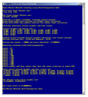 [Click on image for larger view.]
Figure 1. Neural network back-propagation in action.
[Click on image for larger view.]
Figure 1. Neural network back-propagation in action.
A 3-4-2 neural network requires (3*4) + (4*2) = 20 weights and (4+2) = 6 bias values, for a total of 26 weights and bias values. The demo initializes these values to 0.001, 0.002, . . . 0.026 (again, arbitrarily chosen). Back-propagation uses a parameter called the learning rate, and optionally a second parameter called momentum. The demo sets the learning rate to 0.5 and the momentum value to 0.1. These parameters will be explained in detail later, but for now it's enough to say that larger values make the back-propagation training process faster at the risk of missing the best set of weights and bias values.
The demo prepares back-propagation iteration by setting a maximum number of iterations (often called epochs in machine-learning terminology) to 10,000, and an exit condition if the error measure of the difference between computed outputs and target values is less than 0.000010. The demo repeatedly calls the neural network's ComputeOutputs and UpdateWeights methods until an exit condition is reached. In this case, the back-propagation algorithm in method UpdateWeights succeeds in finding a set of weights and bias values that generate outputs (0.12340833, 0.87659517) that are very close (within 0.00000963) to the target values (0.12340000, 0.87660000).
This article assumes you understand basic neural network architecture and the feed-forward mechanism, and that you have at least intermediate-level programming skills with a C-family language. I coded the demo using C#, but you should have no trouble refactoring my code to another language such as Python or Windows PowerShell if you wish. I removed all normal error checking to keep the main ideas of back-propagation as clear as possible. The complete code for the demo program is too long to present in this article, so I focus on the back-propagation algorithm. The complete source code accompanies this article as a download.
Demo Program Structure
The structure of the demo program shown running in Figure 1, with some minor edits and WriteLine statements removed, is presented in Listing 1. I used Visual Studio 2012, but the program has no significant dependencies and any version of Visual Studio will work fine. I created a new C# console application project named BackProp. After the template code loaded, in the Solution Explorer window I renamed the file Program.cs to BackPropProgram.cs, and Visual Studio automatically renamed class Program for me. At the top of the source code, I deleted all references to namespaces except the one to the top-level System namespace.
Listing 1. The demo program structure.
using System;
namespace BackProp
{
  class BackPropProgram
  {
    static void Main(string[] args)
    {
      try
      {
        Console.WriteLine("\nBegin Neural Network training using Back-Propagation demo\n");
        double[] xValues = new double[3] { 1.0, -2.0, 3.0 }; // Inputs
        double[] yValues; // Outputs
        double[] tValues = new double[2] { 0.1234, 0.8766 }; // Target values

        Console.WriteLine("The fixed input xValues are:");
        Helpers.ShowVector(xValues, 1, 8, true);

        Console.WriteLine("The fixed target tValues are:");
        Helpers.ShowVector(tValues, 4, 8, true);

        int numInput = 3;
        int numHidden = 4;
        int numOutput = 2;
        int numWeights = (numInput * numHidden) +
         (numHidden * numOutput) + (numHidden + numOutput);

        BackPropNeuralNet bnn = new BackPropNeuralNet(numInput, numHidden, numOutput);

        Console.WriteLine("\nCreating arbitrary initial weights and bias values");
        double[] initWeights = new double[26] {
          0.001, 0.002, 0.003, 0.004,
          0.005, 0.006, 0.007, 0.008,
          0.009, 0.010, 0.011, 0.012,

          0.013, 0.014, 0.015, 0.016,

          0.017, 0.018,
          0.019, 0.020,
          0.021, 0.022,
          0.023, 0.024,

          0.025, 0.026 };

        Console.WriteLine("\nInitial weights and biases are:");
        Helpers.ShowVector(initWeights, 3, 8, true);

        Console.WriteLine("Loading weights and biases into neural network");
        bnn.SetWeights(initWeights);

        double learnRate = 0.5;
        double momentum = 0.1;
        int maxEpochs = 10000;
        double errorThresh = 0.00001;

        int epoch = 0;
        double error = double.MaxValue;
        Console.WriteLine("\nBeginning training using back-propagation\n");

        while (epoch < maxEpochs) // Train
        {
          yValues = bnn.ComputeOutputs(xValues);
          error = Helpers.Error(tValues, yValues);
          if (error < errorThresh)
          {
            Console.WriteLine("Found weights and bias values at epoch " + epoch);
            break;
          }
          bnn.UpdateWeights(tValues, learnRate, learnRate);
          ++epoch;
        } // Train loop

        double[] finalWeights = bnn.GetWeights();
        Console.WriteLine("Final neural network weights and bias values are:");
        Helpers.ShowVector(finalWeights, 5, 8, true);

        yValues = bnn.ComputeOutputs(xValues);
        Console.WriteLine("\nThe yValues using final weights are:");
        Helpers.ShowVector(yValues, 8, 8, true);

        double finalError = Helpers.Error(tValues, yValues);
        Console.WriteLine("\nThe final error is " + finalError.ToString("F8"));

        Console.WriteLine("\nEnd Neural Network Back-Propagation demo\n");
        Console.ReadLine();
      }
      catch (Exception ex)
      {
        Console.WriteLine("Fatal: " + ex.Message);
        Console.ReadLine();
      }

    } // Main

  } // Program

  public class BackPropNeuralNet { ... }
  public class Helpers { ... }

} // ns
If you compare the code in Listing 1 with the output shown in Figure 1, most of the code in the Main method should be fairly self-explanatory. Class BackPropNeuralNet defines a neural network that can be trained using back-propagation. Class Helpers contains a utility method for convenience (MakeMatrix); display and WriteLine-style debugging (ShowVector, ShowMatrix); and an error function (Error) that measures how close two vectors are, which is used to compare outputs with targets.
The Neural Network Class
The neural network class has quite a few data members, as shown in Listing 2.
Listing 2. The neural network class.
public class BackPropNeuralNet
{
  private int numInput;
  private int numHidden;
  private int numOutput;

  private double[] inputs;
  private double[][] ihWeights; // Input-to-hidden
  private double[] hBiases;
  private double[] hSums;
  private double[] hOutputs;

  private double[][] hoWeights; // Hidden-to-output
  private double[] oBiases;
  private double[] oSums;
  private double[] outputs;

  private double[] hGrads; // Hidden gradients
  private double[] oGrads; // Output gradients


  private double[][] ihPrevWeightsDelta;  // For momentum
  private double[] hPrevBiasesDelta;
  private double[][] hoPrevWeightsDelta;
  private double[] oPrevBiasesDelta;
...
The last six members are associated with the back-propagation training algorithm. Arrays hGrads and oGrads hold so-called gradient values for the hidden-layer neurons (nodes) and output neurons, respectively. Gradients are values that indicate how far away actual output values are from target values. Arrays ihPrevWeightsDelta, hPrevBiasesDelta, hoPrevWeightsDelta and oPrevBiasesDelta are needed for the optional part of the back-propagation algorithm that deals with momentum. Each of these arrays holds a delta value computed from the previous time method UpdateWeights was called.
The neural network is defined assuming that the hyperbolic tangent function is used for hidden layer activation, and the log-sigmoid function is used for output layer activation. In a non-demo scenario, you could add member fields to control how activation is performed in method ComputeOutputs along the lines of:
private string hActivationType; // "log-sigmoid" or "tanh"
private string oActivationType; // "log-sigmoid" or "tanh"
The neural network class constructor sets member variables numInputs, numHidden and numOutputs, and allocates space for all the member arrays and matrices.
The neural network class has five primary methods. Methods SetWeights and GetWeights assign and retrieve the values of a neural network object's weights and bias values. Method GetOutputs retrieves the current values in the outputs array. Method ComputeOutputs accepts an array of input values, copies these values to the class input array, uses the feed-forward mechanism with the current weights and bias values to compute outputs, stores the outputs, and also returns the outputs in an array for convenience. Method ComputeOutputs calls private helper methods SigmoidFunction and HyperTanFunction during the feed-forward activation step. Method UpdateWeights implements one pass of the back-propagation algorithm. The method accepts an array of target values, a learning rate and a momentum value. The method modifies all weights and bias values so that new output values will be closer to the target values. You might want to consider adding a method Train, which encapsulates the training loop code that's in the Main method of the demo program.
Implementing Back-Propagation
The back-propagation algorithm presented in this article involves six steps:
- Compute the so-called gradients for each output-layer node. Gradients are a measure of how far off, and in what direction (positive or negative) the current actual neural network output values are, compared to the target (sometimes called "desired") values.
- Use the output gradient values to compute gradients for each hidden-layer node. Hidden node gradients are computed differently from the output node gradients.
- Use the hidden node gradient values to compute a delta value to be added to input-to-hidden weight.
- Use hidden-node gradient values to compute a delta value for each input-to-hidden bias value.
- Use the output-layer node gradients to compute a delta value for each hidden-to-output weight value.
- Finally, use the output-layer node gradients to compute a delta value for each hidden-to-output bias value.
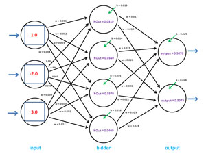
The image in Figure 2 is rather complex, but it will help you understand how back-propagation works. The image shows values before the first call to UpdateWeights for the 3-4-2 demo neural network shown in Figure 1. Recall that the goal is to find weight and bias values so the two neural network outputs are 0.1234 and 0.8766. Initially, the two outputs are 0.5070 and 0.5073 (rounded).
 [Click on image for larger view.]
Figure 2. Computing gradients and deltas.
[Click on image for larger view.]
Figure 2. Computing gradients and deltas.
Method UpdateWeights uses the back-propagation algorithm to adjust neural network weight and bias values:
public void UpdateWeights(double[] tValues, double learn, double mom)
{
  if (tValues.Length != numOutput)
    throw new Exception("target values not same Length as output in UpdateWeights");

  // 1. Compute output gradients. Assumes log-sigmoid
  // 2. Compute hidden gradients. Assumes tanh
  // 3. Update input to hidden weights
  // 4. Update hidden biases
  // 5. Update hidden to output weights
  // 6. Update hidden to output biases
}
Method UpdateWeights assumes that method ComputeOutputs has been called, which places values into the neural network inputs array and the outputs array. Method UpdateWeights is hard-coded to assume that hidden-layer nodes use the hyperbolic tangent activation function and the log-sigmoid activation function. A more flexible design is to store the types of activation functions used at each layer as class members, and pass these values into the class constructor, and then modify the code in method UpdateWeights to branch depending on type of activation function used.
Input parameter tValues is an array that holds the target output values. In the demo program the target values are fixed to 0.1234 and 0.8766. Parameter learn, the learning rate, is a constant that influences how big the changes to weights and bias values are. Parameter mom, for momentum, is a constant that's used to add an additional change to each weight and bias value to speed up the learning process. The values for the learning rate and momentum are typically found by trial and error. Good values vary greatly from problem to problem, but based on my experience, typical values for the learning rate range from 0.3 to 0.7, and typical values for momentum range from 0.01 to 0.2.
The gradient of an output-layer node with a log-sigmoid activation function is equal to (1 - y)(y) * (t - y), where y is the output value of the node and t is the target value. In Figure 2, the gradient for the topmost output node is (1 - 0.5070)(0.5070) * (0.1234 - 0.5070) = -0.0954. A negative value of the gradient means the output value is larger than the target value and weights and bias values must be adjusted to make the output smaller. The gradient of the other output-layer node is (1 - 0.5073)(0.5073) * (0.8766 - 0.5073) = 0.0923.
The (1 - y)(y) term is the calculus derivative of the log-sigmoid function. If you use an activation function that's different from log-sigmoid, you must use the derivative of that function. For example, the calculus derivative of the hyperbolic tangent function is (1 - y)(1 + y). Because the back-propagation algorithm requires the derivative, only functions that have derivatives can be used as activation functions in a neural network if you want to use back-propagation for training. Fortunately, the log-sigmoid and hyperbolic tangent functions -- both of which have very simple derivatives -- can be used in most neural network scenarios.
The code in method UpdateWeights that computes the gradients of the output-layer nodes is:
for (int i = 0; i < oGrads.Length; ++i)
{
  double derivative = (1 - outputs[i]) * outputs[i];
  oGrads[i] = derivative * (tValues[i] - outputs[i]);
}
Computing the gradient of a hidden node is more complicated than computing the gradient of an output-layer node. The gradient of a hidden node depends on the just-computed gradients of all output-layer nodes. The gradient of a hidden node that uses the hyperbolic tangent activation function is equal to (1 - y)(1 + y) * Sum(each output gradient * weight from the hidden node to the output node). Here, y is the output of the hidden node. For example, for the bottommost hidden node in Figure 2 the gradient is (1 - 0.0400)(1 + 0.0400) * (-0.0954 * 0.023) + (0.0923 * 0.024) = about 0.00003 (rounded).
Because computing the back-propagation hidden-layer gradients requires the values of the output-layer gradients, the algorithm computes backward, in a sense -- which is why the back-propagation algorithm is named as it is. The (1 - y)(1 + y) term is the derivative of the hyperbolic tangent. If you use the log-sigmoid function for hidden layer activation, you would replace that term with (1 - y)(y).
The code in method UpdateWeights that computes the gradients of the output-layer nodes is:
for (int i = 0; i < hGrads.Length; ++i)
{
  double derivative = (1 - hOutputs[i]) * (1 + hOutputs[i]);
  double sum = 0.0;
  for (int j = 0; j < numOutput; ++j)
    sum += oGrads[j] * hoWeights[i][j];
  hGrads[i] = derivative * sum;
}
After all the gradient values have been computed, those values are used to update the weights and bias values. Unlike the gradients (which must be computed from right to left in Figure 2), weights and bias values can be computed in any order. And all weights and bias values are computed in the same way, with the minor exception that bias values are computed slightly differently than weight values.
Observe that any neural network weight has an associated from-node and to-node. For example, in Figure 2, weight 0.004 is associated with input-layer node [0] and hidden-layer node [3]. For any input-to-hidden or hidden-to-output weight, a delta value (that is, a value that will be added to the weight to give the new weight) is computed as (gradient of to-node * output of from-node * learning rate). So, the delta for weight 0.004 would be computed as 0.00003 * 3.0 * 0.5 = about 0.000005 (rounded). Here, the 3.0 is the output of the from-node, which is the same as input[0]. The 0.5 is the learning rate. The new value for the weight from input[0] to hidden[3] would be 0.004 + 0.000005.
Notice that the increase in the weight is very small. A small value of the learning rate makes neural network training slow because weights change very little each time through the back-propagation algorithm. A larger value for the learning rate would create a larger delta, which would create a larger change in the weight. But a too-large value for the learning rate runs the risk of the algorithm shooting past the optimal value for a weight or bias.
Most back-propagation algorithms use an optional technique called momentum. The idea is to add an additional increment to the weight in order to speed up training. The momentum term is typically a fixed constant with a value like 0.10 times the value of the previously used delta. If you use momentum in back-propagation, you must store each computed delta value for use in the next training iteration. In Figure 2, suppose the previous weight delta for the weight from input[0] to hidden[3] was 0.000008. Then, after adding the computed delta of 0.000005 to the current weight value of 0.004, an additional (0.000008 * 0.10) = 0.0000008 would be added.
The code in method UpdateWeights that updates the input-to-hidden weights is:
for (int i = 0; i < ihWeights.Length; ++i)
{
  for (int j = 0; j < ihWeights[0].Length; ++j)
  {
    double delta = learn * hGrads[j] * inputs[i];
    ihWeights[i][j] += delta; // update
    ihWeights[i][j] += mom * ihPrevWeightsDelta[i][j]; // add momentum
    ihPrevWeightsDelta[i][j] = delta; // save the delta for next time
  }
}
Notice that the first time method UpdateWeights is called, the values of the four previous-deltas arrays and matrices will all be 0.0 because C# performs implicit array initialization.
The code in method UpdateWeights that updates the hidden-to-output weights is almost identical to the code that updates output-to-hidden weights:
for (int i = 0; i < hoWeights.Length; ++i)
{
  for (int j = 0; j < hoWeights[0].Length; ++j)
  {
    double delta = learn * oGrads[j] * hOutputs[i];
    hoWeights[i][j] += delta;
    hoWeights[i][j] += mom * hoPrevWeightsDelta[i][j];
    hoPrevWeightsDelta[i][j] = delta;
  }
}
Because the neural network class in this article treats and stores bias values as actual biases rather than as special weights with dummy constant 1.0 input values, the bias values must be updated separately. The only difference between updating a bias value and updating a weight value is that there's no output-of-from-node term in the delta. I prefer to add a dummy 1.0 value in the computation of bias deltas to make the code for updating of a bias value symmetric with the code for updating a weight value.
The code in method UpdateWeights that updates the hidden-layer node bias values is:
for (int i = 0; i <hBiases.Length; ++i)
{
  double delta = learn * hGrads[i] * 1.0;
  hBiases[i] += delta;
  hBiases[i] += mom * hPrevBiasesDelta[i];
  hPrevBiasesDelta[i] = delta; // save delta
}
And the code in method UpdateWeights that updates the output-layer node bias values is:
for (int i = 0; i < oBiases.Length; ++i)
{
  double delta = learn * oGrads[i] * 1.0;
  oBiases[i] += delta;
  oBiases[i] += mom * oPrevBiasesDelta[i];
  oPrevBiasesDelta[i] = delta;
}
The implementation of back-propagation presented here should meet most of your needs. One important extension is to modify the code to use a learning rate that varies, rather than a fixed rate. The idea is to start with a relatively high value for the learning rate and then decrease the rate on each iteration through the training loop. Some research suggests this is an effective technique, but using an adaptive learning rate is still being investigated by machine-learning researchers.
Other Considerations
The information presented in this article should give you a solid basis for experimenting with neural-network training using back-propagation. However, modifying the demo program to perform useful prediction would require a lot of work. Topics to implement a realistic neural network prediction system that are not discussed in this article include dealing with multiple input values, encoding and normalizing input data, training error, the train-test and k-fold mechanisms, and choosing activation functions.
Back-propagation is by far the most common neural-network training algorithm, but by no means is it the only algorithm. Important alternatives include real-valued genetic algorithm training and particle swarm optimization training. In general, compared to alternative techniques, back-propagation tends to be the fastest, even though back-propagation can be very slow. In my opinion, the main weakness of back-propagation is that the algorithm is often extremely sensitive to the values used for the learning rate and momentum. For some values, back-propagation may converge quickly to good neural network weights and bias values, but for slightly different values of learning rate and momentum training may not converge at all. This leads to a situation where training a neural network using back-propagation requires quite a bit of trial and error.