Neural Network Lab
Neural Network Cross Entropy Error
To train a neural network you need some measure of error between computed outputs and the desired target outputs of the training data. The most common measure of error is called mean squared error. However, there are some research results that suggest using a different measure, called cross entropy error, is sometimes preferable to using mean squared error.
You can think of a neural network (NN) as a complex function that accepts numeric inputs and generates numeric outputs. The output values for an NN are determined by its internal structure and by the values of a set of numeric weights and biases. The main challenge when working with an NN is to train the network, which is the process of finding the values for the weights and biases so that, for a set of training data with known inputs and outputs, when presented with the training inputs, the computed outputs closely match the known training outputs.
To train an NN you need some measure of error between computed outputs and the desired target outputs of the training data. The most common measure of error is called mean squared error. However, there are some research results that suggest using a different measure, called cross entropy error, is sometimes preferable to using mean squared error.
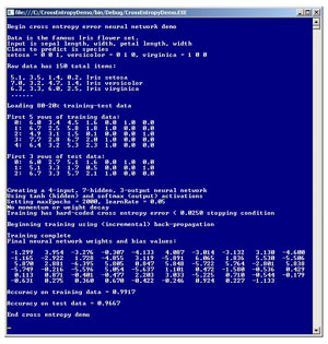
There are many excellent references available that explain the fascinating math behind mean squared error and cross entropy error, but there are few references that explain how to implement NN training using cross entropy error. The best way to see where this article is headed is to take a look at the demo program in Figure 1. The demo program creates an NN that predicts the species of an iris flower (Iris setosa, Iris versicolor or Iris virginica) from sepal (the green part) length and width and petal (the colored part) length and width.
 [Click on image for larger view.]
Figure 1. The Demo Program Predicts the Species of an Iris
[Click on image for larger view.]
Figure 1. The Demo Program Predicts the Species of an Iris
The demo uses a well-known data set called Fisher's iris data. The data set is split randomly into 80 percent (120 items) for training the NN model, and 20 percent (30 items) for testing the accuracy of the model. A 4-7-3 NN is instantiated and then trained using the back-propagation algorithm in conjunction with cross entropy error. After training's completed, the NN model correctly predicted the species of 29 of the 30 (0.9667) test items.
This article assumes you have a solid grasp of neural network concepts, including the feed-forward mechanism and back-propagation algorithm, and that you have at least intermediate-level programming skills, but does not assume you know anything about cross entropy error. The demo is coded using C#, but you should be able to refactor the code to other languages such as JavaScript or Visual Basic .NET without too much difficulty. Most normal error checking has been omitted from the demo to keep the size of the code small and the main ideas as clear as possible.
Cross Entropy Error
The mathematics behind cross entropy (CE) error and its relationship to NN training are very complex, but, fortunately, the results are remarkably simple to understand and implement. CE is best explained by example. Suppose you have just three training items with the following computed outputs and target outputs:
computed       |  target
-------------------------
0.1  0.3  0.6  |  0  0  1
0.2  0.6  0.2  |  0  1  0
0.3  0.4  0.3  |  1  0  0
Using a winner-takes-all evaluation technique, the NN predicts the first two data items correctly because the positions of the largest computed outputs match the positions of the 1 values in the target outputs, but the NN is incorrect on the third data item. The mean (average) squared error for this data is the sum of the squared errors divided by three. The squared error for the first item is (0.1 - 0)^2 + (0.3 - 0)^2 + (0.6 - 1)^2 = 0.01 + 0.09 + 0.16 = 0.26. Similarly, the squared error for the second item is 0.04 + 0.16 + 0.04 = 0.24, and the squared error for the third item is 0.49 + 0.16 + 0.09 = 0.74. So the mean squared error is (0.26 + 0.24 + 0.74) / 3 = 0.41.
Notice that in some sense the NN predicted the first two items with identical accuracy, because for both those items the computed outputs that correspond to target outputs of 1 are 0.6. But observe the squared error for the first two items are different (0.24 and 0.26), because all three outputs contribute to the sum.
The mean (average) CE error for the three items is the sum of the CE errors divided by three. The fancy way to express CE error with a function is shown in Figure 2.
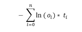 Figure 2. Cross Entropy Error Function
In words this means, "Add up the product of the log to the base e of each computed output times its corresponding target output, and then take the negative of that sum." So for the three items above, the CE of the first item is - (ln(0.1)*0 + ln(0.3)*0 + ln(0.6)*1) = - (0 + 0 -0.51) = 0.51. The CE of the second item is - (ln(0.2)*0 + ln(0.6)*1 + ln(0.2)*0) = - (0 -0.51 + 0) = 0.51. The CE of the third item is - (ln(0.3)*1 + ln(0.4)*0 + ln(0.3)*0) = - (-1.2 + 0 + 0) = 1.20. So the mean cross entropy error for the three-item data set is (0.51 + 0.51 + 1.20) / 3 = 0.74.
Notice that when computing mean cross entropy error with neural networks in situations where target outputs consist of a single 1 with the remaining values equal to 0, all the terms in the sum except one (the term with a 1 target) will vanish because of the multiplication by the 0s. Put another way, cross entropy essentially ignores all computed outputs which don't correspond to a 1 target output. The idea is that when computing error during training, you really don't care how far off the outputs which are associated with non-1 targets are, you're only concerned with how close the single computed output that corresponds to the target value of 1 is to that value of 1. So, for the three items above, the CEs for the first two items, which in a sense were predicted with equal accuracy, are both 0.51.
Using Cross Entropy Error
Although computing cross entropy error is simple, as it turns out it's not at all obvious how to use cross entropy for neural network training, especially in the common scenario where the back-propagation algorithm is used. The back-propagation algorithm computes a term called the gradient for each output node and hidden node. These gradients are a measure of how far off, and in what direction (positive or negative) the current computed outputs are relative to the target outputs. The gradients are then used to adjust the values of the NN's weights and biases so that the computed outputs will be closer to the target outputs.
Exactly how the back-propagation gradients are computed for output nodes is based on some very deep math. This math begins by making an assumption about what type of error needs to be minimized. The computation of the output node gradients therefore depends on whether you want to use mean squared error or mean cross entropy error. The details are very complex but the results are astonishingly simple, and probably best explained with a concrete code example. If you assume you want to minimize mean squared error, the computation of output node gradients can be performed with code like this:
double[] oGrads = new double[numOutput];
for (int i = 0; i < oGrads.Length; ++i)
{
  double derivative = (1 - outputs[i]) * outputs[i];
  oGrads[i] = derivative * (tValues[i] - outputs[i]);
}
Here oGrads is an array to hold the gradient values for each output node. For each gradient, a calculus derivative is computed. In the case of neural networks which perform classification and use softmax activation for the output nodes, the derivative is equal to (1 - y)y where y is the output. This is a consequence of the fact that softmax is a form of the logistic sigmoid function y = 1.0 / (1.0 + e-x). The gradient for a particular node is the value of the derivative times the difference between the target output value and the computed output value.
But if you assume you want to minimize mean cross entropy error, the computation of the output node gradients can be performed with code like this:
double[] oGrads = new double[numOutput];
for (int i = 0; i < oGrads.Length; ++i)
{
  oGrads[i] = tValues[i] - outputs[i];
}
Amazingly, during the complex math algebra behind the scenes, the calculus derivative term cancels out with other terms and you're left with just the difference between target and computed output values. This is one of the most surprising results in all of machine learning. Notice that it isn't necessary to actually compute CE error during training with back-propagation; the computation is implicit rather than explicit.
Cross Entropy Error As a Stopping Condition
Although it isn't required to compute CE error during training with back-propagation, you might want to do so anyway. It will help monitor the progress of training to make sure the process is under control, or to be able to early-exit from the main processing loop when error drops below some small threshold value. For example, the demo program has the code shown in Listing 1.
Listing 1: The Demo Program Code
while (epoch < maxEprochs)
{
  double mcee = MeanCrossEntropyError(trainData);
  if (mcee < 0.025) break;
  Shuffle(sequence); // visit data in random order
  for (int i = 0; i < trainData.Length; ++i) {
    int idx = sequence[i];
    Array.Copy(trainData[idx], xValues, numInput);
    Array.Copy(trainData[idx], numInput, tValues, 0, numOutput);
    ComputeOutputs(xValues);
    UpdateWeights(tValues, learnRate);
  } // Each training tuple
  ++epoch;
}
In the code in Listing 1, the training loop will terminate in at most maxEpochs iterations, and may exit early if the mean CE error drops below 0.0250. Note that the computation of mean CE error is expensive, because all training items must be examined. You might want to compute and check mean error only once every 100 epochs or so, instead.
The code for method MeanCrossEntropyError is presented in Listing 2. The implementation computes CE using the math definition, which results in several multiplications by zero. An alternative is to use an if-then check for target outputs that have a 0.0 value, but you should be cautious when comparing two real values for exact equality.
Listing 2: Computing Mean Cross Entropy Error
private double MeanCrossEntropyError(double[][] trainData)
{
  double sumError = 0.0;
  double[] xValues = new double[numInput];
  double[] tValues = new double[numOutput];

  for (int i = 0; i < trainData.Length; ++i)
  {
    Array.Copy(trainData[i], xValues, numInput); // get inputs
    Array.Copy(trainData[i], numInput, tValues, 0, numOutput); // get targets
    double[] yValues = this.ComputeOutputs(xValues); // compute outputs
    for (int j = 0; j < numOutput; ++j)
    {
      sumError += Math.Log(yValues[j]) * tValues[j]; // CE error
    }
  }
  return -1.0 * sumError / trainData.Length;
}
Mean Squared or Mean Cross Entropy Error?
So, which is better for neural network training: mean squared error or mean cross entropy error? The answer is, as usual, it depends on the particular problem. Research results in this area are rather difficult to compare. If one of the error functions were clearly superior to the other function in all situations, there would be no need for articles like this one. The consensus opinion among my immediate colleagues is that it's best to try mean cross entropy error first; then, if you have time, try mean squared error.
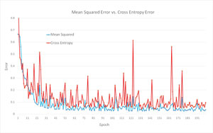
The graph in Figure 3 may give you some insights into the similarities and differences between the two error functions. First, the demo program was run on the 120-item training set using mean squared error. The error values for the first 200 epochs are shown in blue color. Then the demo program was run on the same training set using cross entropy error. Those error values are plotted in red.
 [Click on image for larger view.]
Figure 3. Comparing Mean Squared Error and Mean Cross Entropy Error
[Click on image for larger view.]
Figure 3. Comparing Mean Squared Error and Mean Cross Entropy Error
For this simple example at least, both error functions nicely converged to a small value within 200 epochs. Both demo runs yielded the same accuracy on the test set (29 out of 30 correct). The mean cross entropy error in red shows more volatility than the mean squared error in blue. Higher volatility has both pros (possibly better sensitivity) and cons (possibly increased chance of not converging).
Advantages vs. Disadvantages
Although using CE error is most often used in conjunction with the back-propagation training technique, it's possible to use CE error with the two main training alternatives, particle swarm optimization (PSO) and evolutionary optimization (EO). There's very little published research on the use of CE error with these alternate training algorithms. The few research articles that have been published seem to suggest the advantages and disadvantages of using CE error in conjunction with PSO or EO are similar to the advantages and disadvantages of using CE error with back-propagation. When using CE error with PSO or EO, the computation is explicit rather than implicit (as with back-propagation), so CE is likely to have at least a minor negative impact on training performance.
About the Author
Dr. James McCaffrey works for Microsoft Research in Redmond, Wash. He has worked on several Microsoft products including Azure and Bing. James can be reached at [email protected].