The Data Science Lab
Data Clustering Using R
Find the patterns in your data sets using these Clustering.R script tricks.
Data clustering is the process of programmatically grouping items that are made of numeric components. For example, suppose you have a dataset where each item represents a person's age, annual income and family size. You could cluster the data and examine the results to see if any interesting patterns exist. Data clustering is a fundamental machine learning (ML) exploration technique.
The best way to see where this article is headed is to take a look at the screenshot of a demo R script in Figure 1. The script is named Clustering.R and starts by setting up and displaying a tiny eight-item data set:
(1) 65,220
(2) 73,160
(3) 59,110
(4) 61,120
(5) 75,150
(6) 68,230
(7) 62,130
(8) 66,210
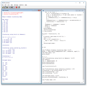 [Click on image for larger view.]
Figure 1. Data Clustering Demo Script
[Click on image for larger view.]
Figure 1. Data Clustering Demo Script
Each data item represents the height (in inches) and weight (in pounds) of a person. The first half of the demo script performs data clustering using the built-in kmeans function. The key result of the call to kmeans is a vector that defines the clustering:
2 1 3 3 1 2 3 2
The number of clusters is set to 3. The indices of the vector (not displayed) indicate the indices of the source data items and the vector values are cluster IDs. So data item (1) belongs to cluster 2, data item (2) belongs to cluster 1, and so, through data item (8), which belongs to cluster 2. (Recall that R vectors use 1-based indexing). The cluster IDs are arbitrary. The important information is the specification of which data items belong to the same cluster.
The second half of the demo script performs clustering using a program-defined function named my_cluster. The result of calling my_cluster is the vector:
2 1 3 3 1 2 3 2
The result clustering is the same as the result of the call to the built-in kmeans function. Because cluster IDs are arbitrary, IDs 1 and 3 could've been swapped giving an equivalent clustering of (2, 3, 1, 1, 3, 2, 1, 2). The script iterates through the clustering vector and displays the source data grouped by cluster:
73  160
75  150
=====
65  220
68  230
66  210
=====
59  110
61  120
62  130
A clear pattern has emerged. There are tall-height, medium-weight people; medium-height, heavy-weight people; and short-height, light-weight people.
In most situations, the built-in kmeans function is quick, simple and effective. However, a custom clustering function can be useful in some scenarios.
In the sections that follow, I'll walk you through the R code that generated the output in Figure 1. After reading this article, you'll have a solid grasp of what data clustering is, how the k-means clustering algorithm works, and be able to write custom clustering code. All of the R code for the demo script is presented in this article. You can also get the code in the download that accompanies this article.
If you want to run the demo script, and you don't have R installed on your machine, installation (and uninstallation) is quick and easy. Do an Internet search for "install R" and you'll find a URL to a page that has a link to "Download R for Windows." I'm using R version 3.3.1, but by the time you read this article, the current version of R may have changed. However, the demo code has no version dependencies, so any recent version of R will work. If you click on the download link, you'll launch a self-extracting executable installer program. You can accept all the installation option defaults, and R will install in about 30 seconds.
To launch the RGui console program, you can double-click on the shortcut item that will be placed by default on your machine's Desktop. Or, you can navigate to directory C:\Program Files\R\R-3.3.1\bin\x64 and double-click on the Rgui.exe file.
Demo Program Structure
To create the demo script, I clicked on the File | New Script option which gave me an untitled script window, shown on the right in Figure 1. Then I clicked on the File | Save As option and saved the (empty) script as Clustering.R in directory C:\ClusteringUsingR.
The structure of the demo script is:
# Clustering.R
my_show_clustered = function(x, clustering, k) { . . }
my_cluster = function(x, k, seed) { . . }
my_dist = function(v1, v2) { . . }
# ===
cat("\nBegin k-means clustering demo \n\n")
...
cat("\nEnd demo \n")
Function my_show_clustered accepts a source data collection as x, a clustering definition vector and the number of clusters as k. The function displays the source data, grouped by cluster. Function my_cluster performs custom clustering using the k-means algorithm. As you'll see shortly, there's a random component to the k-means algorithm. The seed parameter initializes the R system random number generator so that results are reproducible. Function my_dist is a helper method used by my_cluster, and it returns the Euclidean distance between two vectors.
The first few calling statements in the main part of the script are:
cat("\nBegin k-means clustering demo \n\n")
mydf <- read.table("DummyData8.txt", header=F, sep=",")
cat("Raw data: \n")
print(mydf)
The built-in read.table function loads eight comma-delimited data items from file DummyData8.txt -- which has no header -- into a data frame named mydf. The data file is located in the same directory as the source script. If you're new to R, you can think of a data frame as a table that has rows and columns. The data file contents are:
65,220
73,160
59,110
61,120
75,150
68,230
62,130
66,210
The demo script clusters the data using the built-in kmeans function with these statements:
k <- 3
cat("\nClustering using built-in kmeans() \n\n")
obj <- kmeans(mydf, k)
print(obj$cluster)
print(obj$centers)
cat("\n==========\n")
When using the k-means clustering algorithm, and in fact almost all clustering algorithms, the number of clusters, k, must be specified. Like many R functions, kmeans has a large number of optional parameters with default values. After seeing the custom implementation presented in this article, you'll understand exactly what those parameters mean. See the R Documentation page for details.
The demo program doesn't normalize the source data. The purpose of normalizing data before clustering is to prevent columns that have very large magnitudes (for example, annual incomes like 53,000) from dominating columns with small values (like GPA with values such as 3.25). Among my colleagues, there are some differences of opinion about whether data should always be normalized or not. The data could've been normalized using the built-in scale function.
The result of the kmeans function is an object with quite a bit of information. The demo program displays just the vector of cluster IDs and the matrix of cluster centers/means. The means are:
        V1  V2
1 74.00000 155
2 66.33333 220
3 60.66667 120
There are two data items in Cluster 1: (73, 160) and (75, 150). The matrix holds the vector means of the data assigned to each cluster. For example, the mean of cluster 1 is ((73 + 75) / 2, (160 + 150) / 2) = (74.0, 155.0) as shown.
The demo program calls the custom my_cluster function with this code:
clustering <- my_cluster(mydf, k, 3)
cat("\nClustering = \n")
cat(clustering, "\n\n")
cat("Grouped data: \n\n")
my_show_clustered(mydf, clustering, k)
cat("\nEnd demo \n")
The signature of the custom clustering function is similar to the built-in kmeans function except my_cluster accepts a seed value for the R random number generator. Inside the body of the my_cluster function, there's code that displays the means of the clusters.
The Custom Cluster Function
There are many different variations of the k-means algorithm. In very high-level pseudo-code the key ideas are:
initialize k mean vectors
loop
  assign each data item to closest mean (i.e., cluster)
  if no change in clustering, exit loop
  recalculate k means using new clustering
end-loop
return clustering info
The definition of function my_cluster begins with:
my_cluster = function(x, k, seed) {
  set.seed(seed)
  nr <- nrow(x) # num rows
  nc <- ncol(x) # num cols
  ri <- sample(nr, k) # random indices
  means <- x[ri,] # initial means
  rownames(means) <- seq(k)  # renumber
...
To get the algorithm started, the k means are initialized to k random data items selected from the source data. The sample function returns distinct random indices which are then used to initialize a data frame named means. The rownames function is used to renumber the rows in data frame means to 1..k for readability.
Most of the function consists of a while-loop:
...
  clustering <- vector(mode="integer", nr)
  changed <- TRUE
  while(changed == TRUE) {
    changed <- FALSE
    # update clustering
    # update means
  }
  print(means) # optional
  return(clustering)
} # my_cluster
The vector named clustering holds cluster ID assignments. There will be one cluster assignment for each data item. The while-loop will exit when there are no changes to the clustering vector. An alternative design is to add a loop counter and set a maximum number of iterations. In the built-in kmeans function this parameter is named iter.max and has a default value of 10.
The cluster updating code inside the while-loop is:
for (i in 1:nr) {
  mindist <- .Machine$double.xmax  # 1.7e+308
  minindex <- -1
  for (j in 1:k) { # each mean
    d <- my_dist(x[i,],means[j,])
    if (d < mindist) { minindex <- j; mindist <- d }
  }
  oldc <- clustering[i]
  if (minindex != oldc) { changed <- TRUE }
  clustering[i] <- minindex
}
Each data item is examined in turn, and the distance from the data item to each of the k means is calculated using the my_dist helper function. The current item is assigned to the cluster ID that's the index of the mean with the smallest distance.
There are many possible distance functions. The demo uses Euclidean distance. The documentation for the built-in kmeans function doesn't explicitly specify which distance measure is used, but hints that it's squared Euclidean distance. Helper function my_dist is defined:
my_dist = function(v1, v2) {
  sum <- 0.0
  for (i in 1:length(v1)) {
    sum <- sum + (v1[i] - v2[i])^2
  }
  return(sqrt(sum))
}
Euclidean distance between two vectors is the square root of the sum of the differences between vector components. Dropping the sqrt call would give squared Euclidean distance, which would give the same results. One of the peculiarities of the R language is that there are a huge number of functions that operate directly on vectors and matrices. For example, if v1 and v2 are vectors, the expression v1 + v2 adds the vectors component by component without having to use an explicit for-loop. So the body of the function could've been written in one line as:
return( sqrt(sum((v1-v2)^2)) )
For me, when coding in R, it's always a difficult choice when faced with using standard iterative code (which is often easier to understand and debug) versus using high-level code constructions (which is often shorter and better-performing).
The means updating code inside the while-loop is:
newmeans <- matrix(0.0, nrow=k, ncol=nc)
counts <- vector(mode="integer", k)
for (i in 1:nr) {
  cid <- clustering[i] # cluster ID
  newmeans[cid,] <- newmeans[cid,] + as.matrix(x[i,])
  counts[cid] <- counts[cid] + 1
}
newmeans <- newmeans / counts
means <- newmeans
The newmeans matrix accumulates values and the counts vector holds the number of items in each cluster. It's possible, but extremely unlikely, for a count to become zero. You can add an error check for this condition and either return the current clustering or use one of several R error-handling mechanisms.
Displaying Data by Cluster
In some data analysis scenarios it's useful to display data grouped by cluster. The definition of function my_show_clustered begins with:
my_show_clustered = function(x, clustering, k)
{
  nr <- nrow(x) # number rows in source data
  nc <- ncol(x)
...
Here, parameter x is the source data frame, parameter clustering is a vector of cluster IDs and parameter k is the number of clusters. Note that instead of passing in parameter k, k could be determined by finding the largest value in the cluster vector. The function does no error checking.
The body of the function is:
...
  for (cid in 1:k) {
    for (i in 1:nr) {
      if (clustering[i] == cid) {
        for (j in 1:nc) { cat(x[i,j], " ") }
        cat("\n")
      }
    }
    cat("=====\n")
  }
} # function
The function makes k passes through the source data, displaying just data items that belong to cluster k on each pass. An alternative design is to use a single pass through the data and construct a list of data items grouped by cluster ID.
Wrapping Up
As it turns out, the k-means clustering algorithm is very sensitive to the selection of the initial means. If you experiment with the demo code by changing the value of the seed parameter passed to the my_cluster function, you'll observe that every now and then you get obviously bad clustering. There are two main ways to avoid this. The first approach is to use a more sophisticated scheme when initializing the k means so that the means aren't close together. Typically, you try several different sets of initial means and use the set where the means are farthest apart. This approach is what's used in a variation of k-means called the k-means++ algorithm.
The second approach for avoiding a bad clustering result is to run the basic k-means algorithm several times, saving the results, and then analyzing the results to find the set that has the best clustering. The "best" clustering can be measured in several ways because in most real-life data analysis scenarios, there is no clear optimal clustering.
About the Author
Dr. James McCaffrey works for Microsoft Research in Redmond, Wash. He has worked on several Microsoft products including Azure and Bing. James can be reached at [email protected].