The Data Science Lab
Revealing Secrets with R and Factor Analysis
Let's use this classical statistics technique -- and some R, of course -- to get to some of the latent variables hiding in your data.
Factor analysis is a classical statistics technique that examines data that has several variables in order to see if some of the variables are closely connected in some way. One of the standard "Hello World" examples of factor analysis is an examination of user ratings of different films. The idea here is that behind the scenes there are latent, hidden variables, such as movie genre, that explain the observed ratings.
For example, suppose 20 reviewers are asked to assign a rating from one (bad) to five (excellent) to seven different films: "The Hangover," "Meet the Parents," "Forbidden Planet," "Dark City," "Ben Hur," "Gladiator" and "Galaxy Quest." It's possible that reviewers' assigned ratings may be correlated with three latent variables: comedy ("The Hangover" and "Meet the Parents"), science fiction ("Forbidden Planet" and "Dark City") and history ("Ben Hur" and "Gladiator"). Note that "Galaxy Quest" is a film that is both science fiction and comedy.
If in fact a film genre latent variable captures the essence of the ratings data, then you'd be able to guess that a reviewer who liked "Forbidden Planet" and "Dark City" would probably like "Star Wars." Another way you could use factor analysis information is to combine the raw variables that correspond to a latent variable, in order to reduce the dimensionality of the source data.
The best way to see where this article is headed is to take a look at the screenshot of a demo R script in Figure 1. The script is named FactorDemo.R and starts by setting up and displaying a small 20-item data set of film ratings as just described. Next, the demo performs a factor analysis using the built-in (and somewhat unfortunately named) factanal function. The demo script concludes by displaying a graph of the factor analysis. You can clearly see that films are grouped by genre.
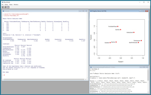 [Click on image for larger view.]
Figure 1. Data Clustering Demo Script
[Click on image for larger view.]
Figure 1. Data Clustering Demo Script
In the sections that follow, I'll walk you through each line of the demo script, and explain how to interpret the results of a factor analysis. After reading this article you should have a good grasp of how to perform a factor analysis using R. All of the R code for the demo script is presented in this article. You can also get the code in the download that accompanies this article.
Setting Up the Source Data
If you want to run the demo script, and you don't have R installed on your machine, installation (and uninstallation) is quick and easy. Do an Internet search for "install R" and you'll find a URL to a page that has a link to "Download R for Windows." I'm using R version 3.3.2, but by the time you read this article, the current version of R may have changed. However, the demo code has no version dependencies, so any recent version of R will work. If you click on the download link, you'll launch a self-extracting executable installer program. You can accept all the installation option defaults, and R will install in about 30 seconds.
To launch the RGui console program, you can double-click on the shortcut item that will be placed by default on your machine's Desktop. Or, you can navigate to directory C:\Program Files\R\R-3.3.2\bin\x64 and double-click on the Rgui.exe file. Because all of the functions needed to run the demo script are included with a default R installation, you don't need to run RGui with administrative privileges (but it is necessary to install optional packages).
To create the demo script, I clicked on the File | New Script option, which gave me an untitled script window, shown on the bottom-right in Figure 1. Then I clicked on the File | Save As option and saved the (empty) script as FactDemo.R in directory C:\FactorAnalysisUsingR.
The first four lines of the demo script are:
# FactDemo.R
# 3.3.2
cat("\nBegin Factor Analysis demo \n\n")
rm(list=ls()))
I comment the name of the script and the R version it was created with. The cat function displays a start-up message, and then I use the rm function to delete all existing objects from the current workspace. Next, I create hardcoded data:
Person <- c("P01", "P02", "P03", "P04", "P05", "P06", "P07",
            "P08", "P09", "P10", "P11", "P12", "P13", "P14",
            "P15", "P16", "P17", "P18", "P19", "P20")
ForbiddenPlanet <- c(4,1,2,4,4,2,3,5,1,3,4,3,2,3,3,1,1,5,5,3)
TheHangover <- c(2,5,1,3,2,4,3,2,5,1,5,2,4,3,2,4,1,5,2,4)
MeetTheParents <- c(3,5,2,5,1,4,4,1,4,2,5,1,4,3,3,4,2,4,1,5)
BenHur <- c(1,1,4,2,5,4,3,2,2,4,2,3,4,3,1,1,5,2,3,4)
Gladiator <- c(2,1,4,2,4,4,3,2,1,5,1,5,4,3,2,3,5,1,5,5)
GalaxyQuest <- c(4,4,1,5,3,3,3,4,3,2,5,3,3,3,3,4,1,5,3,3)
DarkCity <- c(5,3,2,4,4,1,5,4,3,2,5,3,1,3,4,1,2,5,5,3)

mydata <- data.frame(Person,ForbiddenPlanet,TheHangover,
 MeetTheParents,BenHur,Gladiator,GalaxyQuest,DarkCity)
The factanal function can work with several forms of source data. Here, I put the source data into a data frame by creating eight vectors using the tersely named c function and then I pass those vectors to the data.frame function to create a collection named mydata.
In most factor analysis scenarios, you'd read source data from a text file. For example, suppose you had a text file named FilmRatings.txt that looked like:
Person,ForbiddenPlanet, . . . DarkCity
P01,4,2,3,1,2,4,5
P02,1,5,5,1,1,4,3
...
P20,3,4,5,4,5,3,3
Then you could read the data like so:
mydata <- read.table("FilmRatings.txt", header=T, sep=",")
After loading the data, I display part of the data frame, and then create a second data frame that has the non-numeric data removed:
print(head(mydata))
dd <- mydata[,2:8]
The head function selects the first six rows of a table. The statement that creates data frame dd can be interpreted as, "Take all the rows, but just columns 2 through 8 of data frame mydata and place them into a new data frame named dd." Recall that all collections in R use 1-based indexing rather than 0-based indexing. The idea here is to remove the reviewer ID values (P01, P02, etc.) because the factanal function works only with numeric data.
Performing the Factor Analysis
With the source data stored into a data frame, performing a factor analysis can be done with two statements:
mymodel <- factanal(dd, factors=3, rotation="varimax")
print(mymodel)
The factanal function, like most R functions, has many optional parameters. Here, I just use three parameters. The first argument is the source data frame, dd. The second argument is the number of factors to use. In this example, because I specifically created data that has three latent variables, I knew to pass 3 to the factors parameter. I'll explain how to determine the number of factors to use for non-fake data when I explain the analysis output.
The third parameter is rotation and I pass "varimax." This is the default value so I could have omitted the third argument. The rotation parameter can accept a function name that is used behind the scenes, but in ordinary scenarios the default varimax function is fine.
The first part of the output is the Uniqueness section:
Uniquenesses:
ForbiddenPlanet   TheHangover  ...
          0.005         0.092  ...
These values are secondary information and tell you the percentage of the statistical variance for each original variable that isn’t explained by the factors. A large uniqueness value indicates that none of the latent factors captures a variable well, so smaller values are better.
The next part of the output contains the factor Loadings:
Loadings:
                Factor1 Factor2 Factor3
ForbiddenPlanet -0.141   0.987
TheHangover      0.930          -0.205
MeetTheParents   0.798  -0.174  -0.226
BenHur          -0.216  -0.142   0.964
Gladiator       -0.484  -0.182   0.665
GalaxyQuest      0.591   0.557  -0.488
DarkCity                 0.761  -0.273
Notice that "The Hangover" and "Meet the Parents" have large positive values (0.930 and 0.798) for Factor1. This means those two films are very strongly correlated with Factor1 which we know must be the comedy latent variable. Similarly, "Forbidden Planet" and "Dark City" have large loading values for Factor2 (science fiction), and "Ben Hur" and "Gladiator" have large Factor3 (history) loading values. Note that some loading values appear blank (for example, Factor1 for "Dark City"). This just means the values are very close to 0.000, not that the value doesn't exist.
The next part of the output includes the important sum of squares loadings:
               Factor1 Factor2 Factor3
SS loadings      2.151   1.949   1.777
Proportion Var   0.307   0.278   0.254
Cumulative Var   0.307   0.586   0.840
In general, you won't know in advance how many latent variables to specify when performing a factor analysis. There are several ways to determine a good number of latent variables. One of the simplest is to look at the SS loading values and use the rule of thumb that if a value is greater than 1.0 then the factor is significant. This approach is called the Kaiser criterion. In this example, all three SS loading values are greater than 1.0 (2.151, 1.949, 1.777). However, if you perform a factor analysis on some data and get an SS loading value that’s less than 1.0, the factor doesn't work well and so you can try fewer factors.
Note that there’s a limit to the number of factors you can specify. If your data set has v variables and f factors, then (v - f)^2 must be greater than v + f. For the demo data v = 7 so you can specify f = 3 factors because (7 - 3)^2 > (7 + 3), but you can't specify four factors because (7 - 4)^2 is not greater than (7 + 4).
The final part of the output is more secondary information:
Test of the hypothesis that 3 factors are sufficient.
The chi square statistic is 3.77 on 3 degrees of freedom.
The p-value is 0.287
The p-value is the probability that the source data perfectly fits the number of factors specified, so larger values are better. However, it's quite difficult to interpret a factor analysis p-value and in my opinion it's best used to compare two different models.
Graphing the Results
Although it's not necessary, it's sometimes informative to graph the results of a factor analysis. The last four lines of the demo script do that and are:
load <- mymodel$loadings[,1:2]
plot(load, type="p", pch=20, cex=2, col="red", xlim=c(-1.0, 1.0),
  ylim=c(-1.0, 1.4))
text(load, labels=names(dd), pos=2, cex=0.75)
cat("\nEnd demo \n\n")
The first statement fetches the factor loadings for Factor1 and Factor2. Recall that the fields in most R objects can be accessed using the $ operator. Because I'm making a two-dimensional plot, I can only use two of the three factors at a time.
The built-in plot function has a lot of parameters. Here, type="p" means make a point graph. The pch=20 and cex=2 and col="red" mean make red-filled circles that are twice the default size. The xlim and ylim parameters set the limits of the x-axis and y-axis.
The text function adds labels to the graph. The label text is pulled from the header of the dd data frame. I could’ve used shorter names like this:
labels=c("FP", "TH", "MTP", "BH", "G", "GQ", "DC")
The pos=2 argument means place the labels to the left of the data points, and the cex=0.75 means make the label text three-quarters of the default size.
Wrapping Up
Factor analysis essentially aggregates and condenses information. This was quite important in the days before the widespread availability of computers when statistical analyses had to be calculated by hand. Factor analysis is still a useful technique but is now mostly used to simplify the interpretation of data. As the Wikipedia entry on factor analysis points out, the technique is not often used in the fields of physics, biology, and chemistry, but it’s used frequently in fields such as psychology, marketing, and operations research. Once you're aware of what factor analysis is and how it works, you may find valuable applications of the technique with your work data.
About the Author
Dr. James McCaffrey works for Microsoft Research in Redmond, Wash. He has worked on several Microsoft products including Azure and Bing. James can be reached at [email protected].