The Data Science Lab

Neural Network L2 Regularization Using Python

Our data science expert continues his exploration of neural network programming, explaining how regularization addresses the problem of model overfitting, caused by network overtraining.

• By James McCaffrey
• 10/05/2017

Neural network regularization is a technique used to reduce the likelihood of model overfitting. There are several forms of regularization. The most common form is called L2 regularization. If you think of a neural network as a complex math function that makes predictions, training is the process of finding values for the weights and biases constants that define the neural network. The most common way to train a neural network is to use a set of training data with known, correct input values and known, correct output values. You apply an optimization algorithm, typically back-propagation, to find weights and biases values that minimize the error metric between computed output values and the correct output values.

Model overfitting can occur when you train a neural network excessively. This leads to a situation where the trained neural network model predicts the output values in the training data very well, with little error and high accuracy, but when the trained model is applied to new, previously unseen data, the model predicts poorly.

As it turns out, overfitting is often characterized by weights with large magnitudes, such as -20.503 and 63.812, rather than small magnitudes such as 2.057 and -1.004. L2 regularization tries to reduce the possibility of overfitting by keeping the values of the weights and biases small.

To see where this article is headed, look at Figure 1, which shows the screenshot of the run of a demo program. The demo program is coded using Python with the NumPy numeric library, but you should have no trouble refactoring to another language, such as C# or Visual Basic, if you wish to do so. The demo begins by generating synthetic training (200 items) and test data (40 items). Each data item has 10 input predictor variables (often called features) and 4 output variables that represent 1-of-N encoded categorical data. For example, if you were trying to predict the color of an automobile someone will buy, and there were just four color choices, you could encode white as (1, 0, 0, 0), red as (0, 1, 0, 0), silver as (0, 0, 1, 0) and blue as (0, 0, 0, 1).

The demo program creates a neural network with 10 input nodes, 8 hidden processing nodes and 4 output nodes. The number of hidden nodes is a free parameter and must be determined by trial and error. The demo program trains a first model using the back-propagation algorithm without L2 regularization. That first model gives 95.50 percent accuracy on the training data (191 of 200 correct) and 70.00 percent accuracy on the test data (28 of 40 correct).

Then the demo continues by training a second model, this time with L2 regularization. The second model gives 92.00 percent accuracy on the training data (184 of 200 correct) and 72.50 percent accuracy on the test data (29 of 40 correct). In this example, using L2 regularization has made a small improvement in classification accuracy on the test data.

Understanding Neural Network Model Overfitting
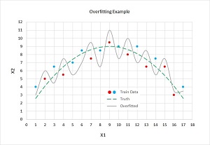
Model overfitting is a significant problem when training neural networks. The idea is illustrated in the graph in Figure 2. There are two predictor variables: X1 and X2. There are two possible categorical classes, indicated by the red (class = 0) and blue (class = 1) dots. You can imagine this corresponds to the problem of predicting if a person is male (0) or female (1), based on normalized age (X1) and normalized income (X2). For example, the left-most data point at (X1 = 1, X2 = 4) is colored blue (female).

The dashed green line represents the true decision boundary between the two classes. This boundary is unknown to you. Notice that data items above the green line are mostly blue (7 of 10) and data items below the green line are mostly red (5 of 7). The five misclassifications in the training data are due to the randomness inherent in almost all real-life data.

A good neural network model would find the true decision boundary represented by the green line. However, if you train a neural network model long enough, it will essentially get too good and generate a model indicated by the solid gray line. The gray line makes perfect predictions on the test data. All the blue dots are above the gray line and all the red dots are below the gray line.

But when the overfitted model is presented with new, previously unseen data, there's a good chance the model will make an incorrect prediction. For example, a new data item at (X1 = 4, X2 = 7) is above the green dashed truth boundary and so it should be classified as blue. But because the data item is below the gray line overfitted boundary, it will be incorrectly classified as red.

If you remember your high school algebra (sure you do!) you might recall that the overfitted gray line, with its jagged shape, resembles the graph of a polynomial function that has large-magnitude coefficients. These coefficients correspond to neural network weights. Therefore, the idea behind L2 regularization is to try to reduce model overfitting by keeping the magnitudes of the weight values small.

Understanding L2 Regularization with Back-Propagation
Briefly, L2 regularization works by adding a term to the error function used by the training algorithm. The additional term penalizes large weight values. The two most common error functions used in neural network training are squared error and cross entropy error. For the rest of this article I'll assume squared error, but the ideas are exactly the same when using cross entropy error. In L2 regularization you add a fraction (often called the L2 regularization constant, and represented by the lowercase Greek letter lambda) of the sum of the squared weight values to the base error. For example, suppose you have a neural network with only three weights. If you set lambda = 0.10 and if the current values of the weights are (5.0, -3.0, 2.0), then in addition to the base squared error between computed output values and correct target output values, the augmented error term adds 0.10 * [ (5.0)^2 + (-3.0)^2 + (2.0)^2 ] = 0.10 * (25.0 + 9.0 + 4.0) = 0.10 * 38.0 = 3.80 to the overall error.

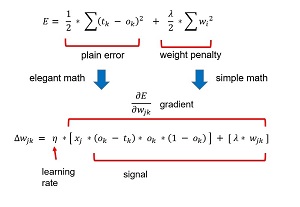
The key math equations (somewhat simplified for clarity) are shown in Figure 3. The top-most equation is squared error augmented with the L2 weight penalty: one-half the sum of the squared differences between the target values and the computed output values, plus one-half a constant lambda times the sum of the squared weight values.

During training, the back-propagation algorithm iteratively adds a weight-delta (which can be positive or negative) to each weight. The weight-delta is a fraction (called the learning rate, usually represented by the lowercase Greek letter eta, η, which resembles a script "n") of the weight gradient. The weight gradient is the calculus derivative of the error function.

Determining the derivative of the base error function requires some very elegant math. But because the derivative of the sum of two terms is just the sum of the derivatives of each term, to use L2 regularization you have to add the derivative of the weight penalty. Luckily, this is quite easy. If you remember introductory calculus, the derivative of y = cx^2 (where c is any constant) is y' = 2cx. In essence the exponent jumps down in front. In the case of the weight penalty term, the exponent 2 cancels the leading one-half term leaving just lambda times the weight. You can see this as the last term in the gradient part of the weight-delta equation.

Let me state that I've "abused notation" greatly here and my explanation is not completely mathematically accurate. But a thorough, rigorous explanation of the relationship between back-propagation and L2 regularization with all of the details would take pages and pages of messy math. Also, the weight-delta equation in Figure 3 is just for hidden-to-output weights. The equation for input-to-hidden weights is a bit more complicated, but the L2 part doesn't change -- you add lambda times the current weight value.

This article isn’t about the back-propagation algorithm, but briefly, in the weight-delta equation, x is the input value associated with the weight being updated (the value of a hidden node). The output minus target term comes from the derivative of the error function, so if you use an error function other than squared error, this term would change. The output times the quantity one minus output term is the derivative of the output layer activation function, which is softmax in the case of neural network classification. So, if you use a different output activation, you'd have to change that term.

If all this seems a bit overwhelming, well, it is. But every person I know who became a more-or-less expert at neural networks learned one thing at a time. Eventually all the parts of the puzzle become crystal clear.

Implementing L2 Regularization
The overall structure of the demo program, with a few edits to save space, is presented in Listing 1.

# nn_L2.py
# Python 3.x

import numpy as np
import random
import math

# helper functions
def showVector(): ...
def showMatrix(): ...
def showMatrixPartial(): ...
def makeData(): ... 
	
class NeuralNetwork: ... 

def main():
  print("Begin L2 demo \n")
  
  print("Generating dummy data")
  genNN = NeuralNetwork(10, 15, 4, 0)
  genNumWts = NeuralNetwork.totalWeights(10,15,4)
  genWeights = np.zeros(shape=[genNumWts], \
    dtype=np.float32)
  genRnd = random.Random(3)
  genWtHi = 9.9; genWtLo = -9.9
  for i in range(genNumWts):
    genWeights[i] = (genWtHi - genWtLo) * \
      genRnd.random() + genWtLo
  genNN.setWeights(genWeights)
  
  dummyTrainData = makeData(genNN, numRows=200, \
    inputsSeed=11) 
  dummyTestData = makeData(genNN, 40, 13) 
  print("Dummy training data: \n")
  showMatrixPartial(dummyTrainData, 4, 1, True) 
   
  numInput = 10
  numHidden = 8
  numOutput = 4
  print("Creating neural network classifier")
  nn = NeuralNetwork(numInput, numHidden, numOutput, seed=0)  
  
  maxEpochs = 500
  learnRate = 0.01
  print("Setting maxEpochs = " + str(maxEpochs))
  print("Setting learning rate = %0.3f " % learnRate)
  
  print("Starting training without L2 regularization")
  nn.train(dummyTrainData, maxEpochs, learnRate)
  print("Training complete")
  
  accTrain = nn.accuracy(dummyTrainData)
  accTest = nn.accuracy(dummyTestData)
  
  print("Accuracy on train, no L2 = %0.4f " % accTrain)
  print("Accuracy on test, no L2 = %0.4f " % accTest)
  
  L2_rate = 0.005
  nn = NeuralNetwork(numInput, numHidden, numOutput, seed=0)
  print("Starting training with L2)
  nn.train(dummyTrainData, maxEpochs, learnRate, \
    L2=True, regRate=L2_rate) 
  print("Training complete")
  
  accTrain = nn.accuracy(dummyTrainData)
  accTest = nn.accuracy(dummyTestData)
  
  print("Accuracy on train with L2 = %0.4f " % accTrain)
  print("Accuracy on test with L2 = %0.4f " % accTest)
  
  print("End demo ")
   
if __name__ == "__main__":
  main()
# end script

The majority of the demo code is an ordinary neural network implemented using Python. The key code that adds the L2 penalty to the hidden-to-output weight gradients is:

for j in range(self.nh):  # each hidden
  for k in range(self.no):  # each output
    hoGrads[j,k] = oSignals[k] * self.hNodes[j]
    if L2 == True:
      hoGrads[j,k] += lamda * self.hoWeights[j,k]

The hoGrads matrix holds hidden-to-output gradients. First, each base gradient is computed as the product of the associated output node signal and the associated input, which is a hidden node value. Then, if the Boolean L2 flag parameter is true, an additional lambda parameter value (spelled as "lamda" to avoid a clash with a Python language keyword) times the current weight is added to the gradient.

The input-to-hidden weight gradients are computed similarly:

for i in range(self.ni):
  for j in range(self.nh):
    ihGrads[i,j] = hSignals[j] * self.iNodes[i]
    if L2 == True:
      ihGrads[i,j] += lamda * self.ihWeights[i,j]

After using L2 regularization to compute gradients, the weights are updated as they would be without L2. For example:

# update input-to-hidden weights
for i in range(self.ni):
  for j in range(self.nh):
    delta = learnRate * ihGrads[i,j]
    self.ihWeights[i,j] += delta

Note that it’s standard practice to not apply the L2 penalty to the hidden node biases or the output node biases. The reasoning is rather subtle, but briefly and informally: A single bias value with large magnitude isn't likely to lead to model overfitting because the bias can be compensated for by multiple associated weights.

An Alternative Approach
If you think carefully about how L2 regularization works, you'll grasp that on each training iteration, each weight is decayed toward zero by a small fraction of the weight's current value. The weight decay toward zero may or may not be counteracted by the other part of the weight gradient.

So, an entirely different approach to simulating the effect of L2 regularization is to not modify the weight gradients at all, and just decay weights by a constant percentage of the current value, followed by a normal weight update. In pseudo-code:

lambda = 0.02
compute gradients in normal non-L2 way
compute weight-deltas in non-L2 way
for-each weight 
  weight = weight * (1 - lambda) # decay by 2%
  weight = weight + delta # normal update
end

This constant decay approach isn’t exactly equivalent to modifying the weight gradients, but it has a similar effect of encouraging weight values to move toward zero.

Wrapping Up
The other common form of neural network regularization is called L1 regularization. L1 regularization is very similar to L2 regularization. The main difference is that the weight penalty term added to the error function is the sum of the absolute values of the weights. This introduces a minor complication because the absolute value function isn’t differentiable everywhere (at w = 0.0 to be exact). I will address L1 regularization in a future article, and I'll also compare L1 and L2. For now, it's enough for you to know that L2 regularization is more common that L1, mostly because L2 usually (but not always) works better than L1.

The whole purpose of L2 regularization is to reduce the chance of model overfitting. There are other techniques that have the same purpose. These anti-overfitting techniques include dropout, jittering, train-validate-test early stopping and max-norm constraints.

• Get Code Download