The Data Science Lab
Linear Regression with R
Now that you've got a good sense of how to "speak" R, let's use it with linear regression to make distinctive predictions.
The R system has three components: a scripting language, an interactive command shell and a large library of mathematical functions that can be used for data analysis. Although R, and its predecessor S, have been around for decades, the use of R has increased dramatically over the past couple of years. R is an open source technology and has been adopted by Microsoft as part of its technology stack.
Perhaps the most fundamental type of R analysis is linear regression. Linear regression can be used for two closely related, but slightly different purposes. You can use linear regression to predict the value of a single numeric variable (called the dependent variable) based on one or more variables that can be either numeric or categorical (called the independent variables). For example, you might want to predict a person's annual income based on their age, political leaning (conservative, moderate, liberal) and years of education.
You can also use R to analyze the strength of the relationship between a single numeric variable (the dependent variable) and one or more numeric variables (the dependent variables). The actual linear regression math is the same whether you want to make a prediction or analyze the strength of a relationship, but it's often useful to make a distinction. In many cases you want to both make a prediction and analyze the strength of the relationship of the variables.
Simple Linear Regression
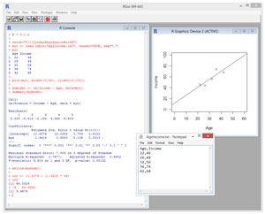
Take a look at the screenshot of a sample R session in Figure 1. The goal of the session is to predict a person's income based on their age. I installed the base R system from r-project.org. I installed version 3.1.2. By the time you read this, the current version of R will likely be different, but the techniques presented in this article have no version dependencies so just about any version of R will work.
The install process is quick and painless. I accepted the default install point of C:\Program Files\R. To launch R, I opened File Explorer and navigated to C:\ProgramFiles\R\R-3.1.2\bin and double-clicked on file Rgui.exe. The R console/shell initially displays some copyright and help information. I cleared the display by typing Ctrl+L.
I used Notepad to create the source data as a simple text file named AgeIncome.txt and saved it at C:\LinearRegressionWithR. The contents of the file are:
Age,Income
22,46
26,44
32,56
36,74
42,68
Data header lines are optional in R but are usually useful. Here, I've placed the dependent variable to predict Income, as the last column, but I could've reversed the order of the columns if I had wanted to. When working with multiple columns of data, I recommend that you place the dependent variable values in the last column.
The first four commands in the session are:
> # v 3.1.2
> setwd("C:\\LinearRegressionWithR")
> myt <- read.table("AgeIncome.txt", header=TRUE, sep=",")
> myt
The > is the R prompt character. The # character begins a comment. The setwd command sets the working directory to the location of the AgeIncome.txt data file so that the file can be referenced without using its full path.
The third command can be interpreted as, "Use the read.table function to store into a data frame (table) object named myt the contents of file AgeIncome.txt where the file has a header line and values are separated by the comma character."
In most cases you can use either the <- or the = operator for assignment. Most of my colleagues and I use <- for object assignment and the = for parameter value assignment. The name of the read.table function might seem a bit odd to you. In most programming languages, multi-word function and variable names are made easier to read by using an underscore or mixed case, such as some_func or someFunc. But R uses the dot character for this name-clarification purpose.
Notice that R functions can use both named parameters (as for header and sep) and positional parameters (AgeIncome.txt for the file parameter). The read.table function has a huge number of optional parameters with default values. This is typical of R functions, but in most cases, like this example, you only need a few parameters.
The fourth command displays the contents of the myt (my table) object simply by typing the name of the object. As an alternative, I could've used print(myt). The advantage of using the print function is that you can specify formatting parameter values.
The next command in the predict-income-from-age session is:
> plot(myt, xlim=c(0,60), ylim=c(0,100))
This command means, "Create a simple x-y graph from the data in data frame myt. For the x-axis (Age) use evenly spaced values from 0 to 60. For the y-axis (Income) use evenly spaced values from 0 to 100." The plot command generates the simple but effective graph in Figure 1, but without the regression line which will be added shortly.
 [Click on image for larger view.]
Figure 1. Predicting Income from Age
[Click on image for larger view.]
Figure 1. Predicting Income from Age
The next two commands perform the linear regression analysis:
> mymodel <- lm(Income ~ Age, data=myt)
> summary(mymodel)
The first command means, "Store into an object named mymodel the results of a linear regression analysis using the data in the data frame table named myt, where Income is the dependent variable and Age is the independent variable." You might have expected "lr" instead of "lm" for the function name. The lm function name stands for "linear model." Linear regression is a subset of techniques called general linear models.
Interpreting the Results
The summary command displays just the basic results of the linear regression analysis, which in most situations is more than enough information. The first part of the summary output is:
Call:
lm(formula = Income ~ Age, data = myt)

Residuals:
     1      2      3      4      5
 2.433 -5.414 -2.185  9.968 -4.803
The function command is echoed back. Notice it includes the positional parameter named formula. There are five residual values, one for each of the five data items in the source data. The residuals are the differences between the actual dependent Income values and the Income values predicted by the linear regression model. For example, for the fourth data item, where is Age = 36, the actual Income of 74 is 9.968 greater than the predicted Income.
The next part of the output is:
Coefficients:
            Estimate Std. Error t value Pr(>|t|)
(Intercept)  11.4076    15.0353   0.759   0.5032
Age           1.4618     0.4643   3.149   0.0513
The values in the Estimate column define the prediction equation. Here, the prediction equation is Income = 11.4076 + (1.4618 * Age). So, if Age = 36, the predicted Income is 11.4076 + (1.4618 * 36) = 64.0324, which is 9.968 less than the actual Income of 74. I'll discuss the rest of the output later when I present a second example.
After the linear regression model was created I added a so-called regression line to the session graph using the command:
> abline(mymodel)
This means, "Add the regression line determined by the model named mymodel to the current graph." The regression line is a visual interpretation of the prediction equation. The regression line is the one line that minimizes the sum of squared deviations from the actual dependent variable values and the predicted dependent variable values. Put another way, the residuals are the deviations. If you square each residual and add all the squared values up you'll get a value that represents error. This error value is the smallest value possible using a straight line model.
The last three commands in the Age-Income session are:
> inc <- 11.4076 + (1.4618 * 36)
> inc
[1] 64.0324
> 74 - 64.0324
[1] 9.9676
>
The first command means, "Store into a variable name inc (income) the result of 11.4076 + (1.4618 * 36)." In other words, the command predicts the income for someone who is 36 years old. The result is 64.0324. The last command calculates the difference between the actual Income value for the 36-year old person, 74, and the predicted Income value. Notice the result of 9.9676 is the residual value for that data item.
Multiple Linear Regression
In linear regression, when there's just a single independent variable, the analysis is sometimes called simple linear regression to distinguish the analysis from situations where there are two or more independent variables. These are sometimes called multiple linear regression analyses.
Suppose you have a data file named AgePoliticEduIncome.txt with contents:
Age,Politic,Edu,Income
20,Mod,12,30
30,Lib,14,32
40,Con,12,50
50,Mod,16,70
60,Lib,16,60
70,Con,12,50
Here, the goal is to predict a person's income from their age, political leaning (Con = conservative, Mod = moderate, Lib = liberal) and years of education. A linear regression analysis session for this problem is shown in Listing 1.
Listing 1: Predicting Income from Age, Political Leaning and Education
> rm(list=ls())
> ls()
character(0)
>
> setwd("C:\\LinearRegressionWithR")
> t <- read.table("AgePoliticEduIncome.txt",
+ header=T, sep=",")
>
> print(t)
  Age Politic Edu Income
1  20     Mod  12     30
2  30     Lib  14     32
3  40     Con  12     50
4  50     Mod  16     70
5  60     Lib  16     60
6  70     Con  12     50
>
> model <- lm(Income ~ Age + Politic + Edu,
+ data=t)
> summary(model)

Call:
lm(formula = Income ~ Age + Politic + Edu, data = t)

Residuals:
     1      2      3      4      5      6
 1.333 -2.667  1.333 -1.333  2.667 -1.333

Coefficients:
             Estimate Std. Error t value Pr(>|t|)
(Intercept) -74.88889   20.70844  -3.616    0.172
Age           0.08889    0.19876   0.447    0.732
PoliticLib  -33.11111    9.72714  -3.404    0.182
PoliticMod  -18.22222    9.32275  -1.955    0.301
Edu          10.00000    2.30940   4.330    0.144

Residual standard error: 4.619 on 1 degrees of freedom
Multiple R-squared:  0.9824, Adjusted R-squared:  0.9121
F-statistic: 13.97 on 4 and 1 DF, p-value: 0.1977

> mydf <- data.frame(Age=20, Politic="Mod", Edu=12)
> predict(model, mydf)
       1
28.66667
>
> mydf <- data.frame(Age=mean(t$Age), Politic="Lib",
+ Edu=13)
> predict(model, mydf)
 1
26
>
> quit()
The first two commands of the multiple regression analysis are:
> rm(list=ls())
> ls()
character(0)
You can interpret the first command, rm(list=ls()), as a magic R incantation to delete all existing objects in the current workspace. The second command means, "Display all objects." The output, character(0), means null or none.
The next three commands load the data into a data frame table, and display the table's contents:
> setwd("C:\\LinearRegressionWithR")
> t <- read.table("AgePoliticEduIncome.txt",
+ header=T, sep=",")
>
> print(t)
Here the value TRUE is specified using the shortcut form T. The default separator is whitespace so the sep argument is required here. Many R commands can be very long. When typing a long command, you can hit the enter key in the middle of the command and R will respond with a "+" prompt indicating that your command is not yet complete. The data in table t (the name is allowed, but not very good style, because R is case-sensitive) is displayed using the print function.
The linear regression model is created and displayed with these two commands:
> model <- lm(Income ~ Age + Politic + Edu, data=t)
> summary(model)
The formula argument of Income ~ Age + Politic + Edu means, "Create a linear regression model where Income is the dependent variable, and Age, Politic, and Edu are the dependent variables. The "+" sign here is just R formula syntax and doesn't indicate addition. An alternate approach for loading a data frame that you'll often see in old examples omits the explicit data=<table> parameter in the lm function call, but then adds a second command using the attach function, for example, attach(t). I do not recommend using the attach function because it can, and often does, create object name clashes.
Interpreting the Output of Multiple Regression
The output in the Coefficients section may seem confusing at first glance and requires some explanation:
             Estimate
(Intercept) -74.88889
Age           0.08889
PoliticLib  -33.11111
PoliticMod  -18.22222
Edu          10.00000
There are entries for the numeric Age and Edu variables as you'd expect, but instead of a single Politic variable, there are PoliticLib and PoliticMod. You can guess, correctly, that these stand for liberal and moderate values, but there is no corresponding PoliticCon variable.
In the case of categorical variables, R encodes each value using what's called 1-of-(N-1) encoding. Here, there are N = 3 possible values, Mod, Lib, Con. The first value encountered in the source data, Mod, gets mapped to what you can think of as a Boolean variable named PoliticMod where if the actual categorical value is Mod, then PoliticMod is set to 1, otherwise (if the value is Lib or Con) PoliticMod is set to 0. The encoding is similar for the second data value encountered, Lib, resulting in a PoliticLib variable.
You'd expect there to be a third variable named PoliticCon, however, for interesting mathematical reasons, creating Boolean-like variables for all N categorical values of a categorical variable leads to an error condition called multicollinearity.
So, suppose you want to predict the income for a person who is 20 years old, is a moderate politically and has 14 years of education. The predicted income is calculated as income = -74.89 + (0.89 * 20) + (-33.11 * 0) + (-18.22 * 1) + (10.00 * 14). If you wanted to predict the income for a 20-year-old, who is conservative and has 14 years of education, the predicted income is calculated as income = -74.89 + (0.89 * 20) + (-33.11 * 0) + (-18.22 * 0) + (10.00 * 14).
Because R encodes the first N-1 categorical values encountered in the source data, that means you can get different model coefficient values depending on the order of the items in the source data. However, no matter how the data is ordered, the resulting models will be mathematically equivalent.
In the output, the values in Std. Error, t, and the Pr(>|t|) columns are a bit too complicated to explain in detail in this article. Briefly, and loosely speaking, the standard error values give a measure of how variable the coefficients are. The t and Pr(>|t|) values indicate the importance of each independent variable, where smaller values for Pr are better, meaning the variable is important.
Similarly, the interpretation of the other values in the output -- residual standard error, multiple R-squared, adjusted R-squared, F-statistic and p-value -- are a bit outside the scope of this article. Briefly, the two R values and the p-value all indicate how well the model fits the data. An R value of 1.0 means a perfect fit and a p-value of 0.0 means a perfect fit.
Making Predictions
In R you can use the predict function to make predictions. In Listing 1, the two commands to make a prediction are:
> mydf <- data.frame(Age=20, Politic="Mod", Edu=12)
> predict(model, mydf)
       1
28.66667
The first commands means, "Create a data frame object named mydf where the Age variable is set to 20, Politic is set to Mod, and Edu is set to 12." The second commands means, "Predict the value of the dependent variable (Income) using the information in the linear regression model named model and input values supplied by the data frame named mydf." Notice the input values correspond exactly to the first data item. The predicted income is 28.66667.
Next, the session predicts the income for a hypothetical person not in the original data set:
> mydf <- data.frame(Age=mean(t$Age), Politic="Lib", Edu=13)
> predict(model, mydf)
 1
26
The predicted income is 26.00. Notice the Age value is specified using the R mean (arithmetic average) function. The notation t$Age means, "the Age values in data frame t." The $ character is used to specify columns.
Parting Comments
For many of my colleagues, one of the most difficult aspects of data analysis is not actually performing the analysis, but rather, knowing when to use a particular statistical technique. When I'm trying to determine which R technique to use, I start by mentally imagining the source data in an Excel spreadsheet. If there is one column that I'm particularly interested in, and that column is strictly numeric, and the other columns are either numeric or categorical, then linear regression is a good place to start.
It is possible to perform linear regression analyses using R in situations where the variable of interest is categorical. However, in my opinion, there are other techniques that are preferable in such scenarios.