The Data Science Lab
Logistic Regression Using Python
The data doctor continues his exploration of Python-based machine learning techniques, explaining binary classification using logistic regression, which he likes for its simplicity.
The goal of a binary classification problem is to predict a class label, which can take one of two possible values, based on the values of two or more predictor variables (sometimes called features in machine language terminology). For example, you might want to predict the sex (male = 0, female = 1) of a person based on their age, annual income and height.
There are many different ML techniques you can use for binary classification. Logistic regression is one of the most common. Logistic regression is best explained by example. Continuing the example above, suppose a person has age = x1 = 3.5, income = x2 = 5.2 and height = x3 = 6.7 where the predictor x-values have been normalized so they roughly have the same scale (a 35-year old person who makes $52,000 and is 67 inches tall). And suppose the logistic regression model is defined with b0 = -9.71, b1 = 0.25, b2 = 0.47, b3 = 0.51.
To make a prediction, you first compute a z value:
z = b0 + (b1)(x1) + (b2)(x2) + (b3)(x3)
   = -9.71 + (0.25)(3.5) + (0.47)(5.2) + (0.51)(6.7)
   = -0.484
Then you use the z value to compute a p value:
p = 1.0 / (1.0 + e^(-z))
   = 0.3813
Here e is Euler's number (approximately 2.71828). It's not obvious, but the p value will always be between 0 and 1. If the p value is less than 0.5, the prediction is class label 0. If the p value is greater than 0.5, the prediction is class label 1. For the example, because p is less than 0.5, the prediction is "male."
OK, but where do the b0, b1, b2 and b3 values come from? To determine the b values, you obtain training data that has known predictor x values and known class label y values. Then you use one of many possible optimization algorithms to find values for the b constants so that the computed p values closely match the known, correct y values.
This article explains how to implement logistic regression using Python. There are several machine learning libraries that have built-in logistic regression functions, but using a code library isn't always feasible for technical or legal reasons. Implementing logistic regression from scratch gives you full control over your system and gives you knowledge that can enable you to use library code more effectively.
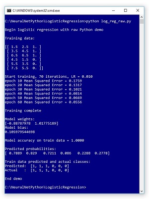
A good way to see where this article is headed is to take a look at the screenshot of a demo program in Figure 1 and the associated data shown in the graph in Figure 2. The demo program sets up six dummy training items. Each item has just two predictor variables for simplicity and so that the training data can be visualized easily. The training data is artificial, but you can think of it as representing the normalized age and income of a person. There are three data items that are class 0 and three items that are class 1.
The demo program trains the logistic regression model using an iterative process. Behind the scenes, the demo is using the gradient ascent log likelihood optimization technique (which, as you'll see, is much easier than it sounds). After training, the demo displays the b0 value, sometimes called the bias, and the b1 and b2 values, sometimes called weights.
 [Click on image for larger view.]
Figure 1 Logistic Regression Demo in Action
[Click on image for larger view.]
Figure 1 Logistic Regression Demo in Action
The demo concludes by displaying the computed p values and the associated y values for each of the six training items. The demo logistic regression model correctly predicts the class labels of all six training items, which shouldn't be too much of a surprise because the data is so simple.
 [Click on image for larger view.]
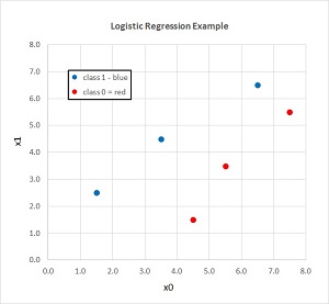
Figure 2. The Demo Training Data
[Click on image for larger view.]
Figure 2. The Demo Training Data
This article assumes you have intermediate or better coding ability with a C-family language, but does not assume you know anything about logistic regression. The demo program is coded using Python, but you shouldn't have too much trouble refactoring the code to another language. The demo program is a bit too long to entirely present presented in this article, and the complete source code is available in the accompanying file download.
Overall Demo Program Structure
The overall demo program structure, with a few minor edits to save space, is presented in Listing 1. To edit the demo program, I used Notepad. Most of my colleagues prefer using one of the many nice Python editors that are available.
I named the program log_reg_raw.py where the "raw" is intended to indicate that the program uses raw Python version 3 without any external ML libraries. The demo program begins by importing the NumPy library. The demo uses the Anaconda distribution of Python 3, but there are no significant version dependencies so any version of Python 3 with NumPy will work fine.
Listing 1: Overall Program Structure
# log_reg_raw.py
# Python + NumPy logistic regression

import numpy as np

# helper functions
def ms_error(data, W, b):
def accuracy(data, W, b):
def pred_probs(data, W, b):
def pred_y(pred_probs):

def main():
  print("Begin logistic regression demo ")

  np.random.seed(0)

  train_data = np.empty(shape=(6,3), dtype=np.float32)
  train_data[0] = np.array([1.5, 2.5, 1])
  train_data[1] = np.array([3.5, 4.5, 1])
  train_data[2] = np.array([6.5, 6.5, 1])
  train_data[3] = np.array([4.5, 1.5, 0])
  train_data[4] = np.array([5.5, 3.5, 0])
  train_data[5] = np.array([7.5, 5.5, 0])

  print("Training data: ")
  print(train_data)

  W = np.random.uniform(low = -0.01, high=0.01, size=2)
  b = np.random.uniform(low = -0.01, high=0.01)

  # train code here
  print("Training complete ")

  print("Model weights: ")
  print(W)
  print("Model bias:")
  print(b)
  print("")

  acc = accuracy(train_data, W, b)
  print("Model accuracy on train data = %0.4f " % acc)

  pp = pred_probs(train_data, W, b)
  np.set_printoptions(precision=4)
  print("Predicted probabilities: ")
  print(pp)

  preds = pred_y(pp)
  actuals = [1 if train_data[i,2] == 1 else \
    0 for i in range(len(train_data))]
  print("Train data predicted and actual classes:")
  print("Predicted: ", preds)
  print("Actual   : ", actuals)

  print("End demo ")

if __name__ == "__main__":
  main()

# end script
The main function begins by setting up hard-coded training data:
np.random.seed(0)
train_data = np.empty(shape=(6,3), dtype=np.float32)
train_data[0] = np.array([1.5, 2.5, 1])
train_data[1] = np.array([3.5, 4.5, 1])
train_data[2] = np.array([6.5, 6.5, 1])
train_data[3] = np.array([4.5, 1.5, 0])
train_data[4] = np.array([5.5, 3.5, 0])
train_data[5] = np.array([7.5, 5.5, 0])
The NumPy random seed is set to 0 so that the demo results are reproducible. The demo places the correct class 0/1 label values at the end of each training item, which is a bit more common than placing the label values at the beginning.
In a non-demo scenario, instead of hard-coding the data, you'd likely read data from a text file, for example:
train_data = np.loadtxt("my_data.txt",
  dtype=np.float32, delimiter=",")
The demo sets up the b0 bias value and the b1 and b2 weight values by initializing them to random values between -0.01 and +0.01:
W = np.random.uniform(low = -0.01, high=0.01, size=2)
b = np.random.uniform(low = -0.01, high=0.01)
Most of the demo code is related to training the logistic regression model to find good values for the W weights and the b bias. The training code will be explained in the next section of this article. After training has completed, the demo program displays the resulting weights and bias values and the classification accuracy of the model:
print("Training complete ")
print("Model weights: ")
print(W)
print("Model bias:")
print(b)
acc = accuracy(train_data, W, b)
print("Model accuracy on train data = %0.4f " % acc)
During training, you are concerned with model error but after training completes, the relevant metric is classification accuracy, which is just the percentage of correct predictions.
Next, the demo uses the weights and bias values to compute and display the raw p values:
pp = pred_probs(train_data, W, b)
np.set_printoptions(precision=4)
print("Predicted probabilities: ")
print(pp)
Printing the raw p values is optional but useful for debugging and also points out that if you write logistic regression from scratch, you have complete control over your system.
The main function concludes by using the raw p values to compute and display the predicted class 0/1 label values. The actual class labels are also pulled from the training data and displayed:
. . .
  preds = pred_y(pp)
  actuals = [1 if train_data[i,2] == 1 else \
    0 for i in range(len(train_data))]
  print("Train data predicted and actual classes:")
  print("Predicted: ", preds)
  print("Actual   : ", actuals)
  print("End demo ")
if __name__ == "__main__":
  main()
# end script)
Pulling the actual class label values from the training data matrix uses a Python shortcut. A more traditional style would be something like:
actuals = []
for i in range(0, len(train_data)):
  if train_data[i,2] == 0:
    actuals.insert(i,0)
  else:
    actuals.insert(i,1)
Python has many terse one-line syntax shortcuts because the language was designed to be used interactively.
Training the Logistic Regression Model
Training the model begins by setting up the maximum number of training iterations and the learning rate:
lr = 0.01
max_iterations = 70
indices = np.arange(len(train_data))
print("Start training, %d iterations,\
  LR = %0.3f " % (max_iterations, lr))
for iter in range(0, max_iterations):
  . . .
The maximum number of training iterations to use and the learning rate (lr) will vary from problem to problem and must be determined by trial and error. The indices array initially holds values (0, 1, 2, 3, 4, 5). During training, the indices array is shuffled and used to determine the order in which each training data item is processed:
np.random.shuffle(indices)
for i in indices:  # each training item
  X = train_data[i, 0:2]  # inputs
  z = 0.0
  for j in range(len(X)):
    z += W[j] * X[j]
  z += b
  p = 1.0 / (1.0 + np.exp(-z))
  . . .
The z value for each training item is calculated as the sum of the products of each weight value and the associated predictor value, as described previously. The bias value is then added. Then, the z value is used to compute the p value. The computation of p as 1.0 / (1.0 + e^(-z)) is called the logistic sigmoid function, and this is why logistic regression is named as it is.
Next, each weight value and the bias value are updated:
for j in range(0, 2):
  W[j] += lr * X[j] * (y - p)
b += lr * (y - p)
The update computation is short but not obvious. The logic is very deep. What is being used is called gradient ascent log likelihood maximization. The term (y - p) is the difference between a target value and a computed p value. Suppose the target y value is 1 and the computed p value is 0.74. You want the value of p to increase so that it is closer to y. The (y - p) term will be 1 - 0.74 = 0.26. You take this delta, multiply by the associated input value x (to take care of the sign of the input value), then multiply by a small fraction called the learning rate. The result is added to the weight being processed and then the computed p will get a bit closer to the target y. Very clever!
During training, it's important to monitor the average error between computed p values and target y values so you can spot problems:
. . .
  if iter % 10 == 0 and iter > 0:
    err = ms_error(train_data, W, b)
    print("epoch " + str(iter) +
      " Mean Squared Error = %0.4f " % err)
print("Training complete ")
The demo program computes the mean squared error between y and p using helper function ms_error. For example, if in one training item, the target y is 1 and the computed p is 0.74, then the squared error for the data item is just (1 - 0.74)^2 = 0.26 * 0.26 = 0.0676. The mean squared error is the average of the error values across all training items.
Wrapping Up
The primary advantage of logistic regression is simplicity. However, the major disadvantage of logistic regression is that it can only work well with data that is mostly linearly separable. For example, in the graph in Figure 2, if a training point with class label 0 (red) was added at (2.5, 3.5), no line could be drawn so that all the red dots are on one side of the classification boundary and all the blue dots are on the other side. That said, much real-life data is mostly linearly separable, and in such situations logistic regression can work well.
Logistic regression can in principle be modified to handle problems where the item to predict can take one of three or more values instead of just one of two possible values. The is sometimes called multi-class logistic regression. But in my opinion, using an alternative classification technique, a neural network classifier, is a better option.
Logistic regression can handle non-numeric predictor variables. The trick is to encode such variables using what is called 1-of-(N-1) encoding. For example, if a predictor variable is color, with possible values (red, blue, green), then you'd encode red as (1, 0), blue as (0, 1) and green as (-1, -1).
The demo program uses gradient accent log likelihood maximization to train the logistic regression model. There are many other approaches including gradient descent error minimization, iterated Newton-Raphson, swarm optimization and L-BFGS optimization. In my opinion, all these alternative techniques produce roughly equivalent results, but the gradient ascent technique is simpler.
About the Author
Dr. James McCaffrey works for Microsoft Research in Redmond, Wash. He has worked on several Microsoft products including Azure and Bing. James can be reached at [email protected].