The Data Science Lab
Simulated Annealing Optimization Using C# or Python
Dr. James McCaffrey of Microsoft Research shows how to implement simulated annealing for the Traveling Salesman Problem (find the best ordering of a set of discrete items).
The goal of a combinatorial optimization problem is to find the best ordering of a set of discrete items. A classic combinatorial optimization challenge is the Traveling Salesman Problem (TSP). The goal of TSP is to find the order in which to visit a set of cities so that the total distance traveled is minimized.
One of the oldest and simplest techniques for solving combinatorial optimization problems is called simulated annealing. This article shows how to implement simulated annealing for the Traveling Salesman Problem using C# or Python.
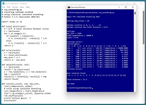
A good way to see where this article is headed is to take a look at the screenshot of a demo program in Figure 1. The demo sets up a synthetic problem where there are 20 cities, labeled 0 through 19. The distance between cities is designed so that the best route starts at city 0 and then visits each city in order. The total distance of the optimal route is 19.0.
The demo sets up simulated annealing parameters of max_iter = 2500, start_temperature = 10000.0 and alpha = 0.99. Simulated annealing is an iterative process and max_iter is the maximum number of times the processing loop will execute. The start_temperature and alpha variables control how the annealing process explores possible solution routes.
The demo sets up a random initial guess of the best route as [ 7, 11, 6 . . 17, 3 ]. After iterating 2500 times, the demo reports the best route found as [ 0, 1, 2, 3, 4, 5, 6, 7, 9, 8, 10, 11, 12, 13, 14, 15, 16, 17, 18, 19 ]. The total distance required to visit the cities in this order is 21.5 and so the solution is close to, but not quite as good as, the optimal solution (the order of cities 8 and 9 is reversed).
 [Click on image for larger view.] Figure 1: Simulated Annealing to Solve the Traveling Salesman Problem.
This article assumes you have an intermediate or better familiarity with a C-family programming language, preferably C# or Python, but does not assume you know anything about simulated annealing. The complete source code for the demo program is presented in this article, and the code is also available in the accompanying file download.
Understanding Simulated Annealing
Suppose you have a combinatorial optimization problem with just five elements, and where the best ordering/permutation is [B, A, D, C, E]. A primitive approach would be to start with a random permutation such as [C, A, E, B, D] and then repeatedly swap randomly selected pairs of elements until you find the best ordering. For example, if you swap the elements at [0] and [1], the new permutation is [A, C, E, B, D].
This approach works if there are just a few elements in the problem permutation, but fails for even a moderate number of elements. For the demo problem with n = 20 cities, there are 20! possible permutations = 20 * 19 * 18 * . . * 1 = 2,432,902,008,176,640,000. That's a lot of permutations to examine.
Expressed as pseudo-code, simulated annealing is:
make a random initial guess
set initial temperature
loop many times
  swap two randomly selected elements of the guess
  compute error of proposed solution
  if proposed solution is better than curr solution then
    accept the proposed solution
  else if proposed solution is worse then
    accept the worse solution anyway with small probability
  else
    don't accept the proposed solution
  end-if
  reduce temperature slightly
end-loop
return best solution found
By swapping two randomly selected elements of the current solution, an adjacent proposed solution is created. The adjacent proposed solution will be similar to the current guess so the search process isn't random. A good current solution will likely lead to a good new proposed solution.
By sometimes accepting a proposed solution that's worse than the current guess, you avoid getting trapped into a good but not optimal solution. The probability of accepting a worse solution is given by:
accept_p = exp((err - adj_err) / curr_temperature)
where exp() the mathematical exp() function, err is the error associated with the current guess, adj_err is the error associated with the proposed adjacent solution, and curr_temperature is a value such as 1000.0. In simulated annealing, the temperature value starts out large, such as 10000.0 and then is reduced slowly on each iteration. Early in the algorithm, when temperature is large, accept_p will be large (close to 1) and the algorithm will often move to a worse solution. This allows many permutations to be examined. Late in the algorithm, when temperature is small, accept_p will be small (close to 0) and the algorithm will rarely move to a worse solution.
The computation of the acceptance probability is surprisingly tricky. In the demo program, the acceptance probability is computed when adjacent error is larger (worse) than the current error, and so the numerator term (err - adj_err) is less than 0. As the value of the current temperature decreases, dividing by the current temperature makes the fraction become more negative, which is smaller. Taking the exp() of smaller values gives smaller values. In short, as the temperature value decreases, the acceptance probability decreases. Here's an example:
err   adj_err  temp     accept_p
50    60       10000    0.999000
50    60        1000    0.990050
50    60         100    0.904837
50    60          10    0.367879
50    60           1    0.000045
It's very easy to botch computing the acceptance probability. For example, if you have a combinatorial optimization problem where the goal is to maximize some value, rather than minimize an error, you need to reverse the order of the terms in the numerator.
The temperature reduction is controlled by the alpha value. Suppose temperature = 1000.0 and alpha = 0.90. After the first processing iteration, temperature becomes 1000.0 * 0.90 = 900.0. After the next iteration temperature becomes 900.0 * 0.90 = 810.0. After the third iteration temperature becomes 810.0 * 0.90 = 729.0. And so on. Smaller values of alpha decrease temperature more quickly.
There are alternative ways you can decrease the temperature. Instead of using an alpha reduction factor, one common approach is to multiply a fixed starting temperature by the fraction of the remaining iterations. When there are many iterations remaining, the temperature will be large. When there are few iterations remaining, the temperature will be small.
The Demo Program
The complete demo program Python code, with a few minor edits to save space, is presented in Listing 1. I indent using two spaces rather than the standard four spaces. The backslash character is used for line continuation to break down long statements.
Listing 1: The Simulated Annealing for TSP Python Program
# tsp_annealing.py
# traveling salesman problem
# using classical simulated annealing
# Python 3.7.6 (Anaconda3 2020.02)

import numpy as np

def total_dist(route):
  d = 0.0  # total distance between cities
  n = len(route)
  for i in range(n-1):
    if route[i] < route[i+1]:
      d += (route[i+1] - route[i]) * 1.0
    else:
      d += (route[i] - route[i+1]) * 1.5
  return d

def error(route):
  n = len(route)
  d = total_dist(route)
  min_dist = n-1
  return d - min_dist

def adjacent(route, rnd):
  n = len(route)
  result = np.copy(route)
  i = rnd.randint(n); j = rnd.randint(n)
  tmp = result[i]
  result[i] = result[j]; result[j] = tmp
  return result

def solve(n_cities, rnd, max_iter,
  start_temperature, alpha):
  # solve using simulated annealing
  curr_temperature = start_temperature
  soln = np.arange(n_cities, dtype=np.int64)
  rnd.shuffle(soln)
  print("Initial guess: ")
  print(soln)

  err = error(soln)
  iteration = 0
  interval = (int)(max_iter / 10)
  while iteration < max_iter and err > 0.0:
    adj_route = adjacent(soln, rnd)
    adj_err = error(adj_route)

    if adj_err < err:  # better route so accept
      soln = adj_route; err = adj_err
    else:          # adjacent is worse
      accept_p = \
        np.exp((err - adj_err) / curr_temperature)
      p = rnd.random()
      if p < accept_p:  # accept anyway
        soln = adj_route; err = adj_err
      # else don't accept

    if iteration % interval == 0:
      print("iter = %6d | curr error = %7.2f | \
      temperature = %10.4f " % \
      (iteration, err, curr_temperature))

    if curr_temperature < 0.00001:
      curr_temperature = 0.00001
    else:
      curr_temperature *= alpha
    iteration += 1

  return soln

def main():
  print("\nBegin TSP simulated annealing demo ")

  num_cities = 20
  print("\nSetting num_cities = %d " % num_cities)
  print("\nOptimal solution is 0, 1, 2, . . " + \
    str(num_cities-1))
  print("Optimal solution has total distance = %0.1f " \
    % (num_cities-1))
  rnd = np.random.RandomState(4)
  max_iter = 2500
  start_temperature = 10000.0
  alpha = 0.99

  print("\nSettings: ")
  print("max_iter = %d " % max_iter)
  print("start_temperature = %0.1f " \
    % start_temperature)
  print("alpha = %0.2f " % alpha)

  print("\nStarting solve() ")
  soln = solve(num_cities, rnd, max_iter,
    start_temperature, alpha)
  print("Finished solve() ")

  print("\nBest solution found: ")
  print(soln)
  dist = total_dist(soln)
  print("\nTotal distance = %0.1f " % dist)

  print("\nEnd demo ")

if __name__ == "__main__":
  main()
The demo program is structured so that all the control logic is in a main() function. The main() begins by setting up parameters for simulated annealing:
import numpy as np
def main():
  print("Begin TSP simulated annealing demo ")
  num_cities = 20
  print("Setting num_cities = %d " % num_cities)
  print("Optimal solution is 0, 1, 2, . . " + \
    str(num_cities-1))
  print("Optimal solution has total distance = %0.1f " \
    % (num_cities-1))
  rnd = np.random.RandomState(4)
  max_iter = 2500
  start_temperature = 10000.0
  alpha = 0.99
. . .
The program uses a local RandomState object rather than the numpy global object. This makes it easier to make program runs reproducible. The seed value of 4 was used only because it gave representative results. Finding good values for the max_iter, start_temperature and alpha variables is a matter of trial and error. Simulated annealing is often very sensitive to these values which makes tuning difficult. The difficulty of parameter tuning is the biggest weakness of simulated annealing.
Next, the demo echoes the parameter values:
  print("\nSettings: ")
  print("max_iter = %d " % max_iter)
  print("start_temperature = %0.1f " % start_temperature)
  print("alpha = %0.2f " % alpha)
The demo passes the simulated annealing parameters to a program-defined solve() function:
  print("Starting solve() ")
  soln = solve(num_cities, rnd, max_iter,
    start_temperature, alpha)
  print("Finished solve() ")
The demo concludes by displaying the result:
  print("Best solution found: ")
  print(soln)
  dist = total_dist(soln)
  print("Total distance = %0.1f " % dist)
  print("End demo ")
if __name__ == "__main__":
  main()
Computing Distance Traveled
The demo defines a function that computes the total distance traveled for a specified route that visits all 20 cities:
def total_dist(route):
  d = 0.0  # total distance between cities
  n = len(route)
  for i in range(n-1):
    if route[i] < route[i+1]:
      d += (route[i+1] - route[i]) * 1.0
    else:
      d += (route[i] - route[i+1]) * 1.5
  return d
For any pair of from-to cities (A, B), if A is less than B then the distance between the two cities is 1.0 * (B - A). For example, the distance from city 4 to city 11 is 7.0. If B is less than A then the distance between cities is 1.5 * (A - B). For example, the distance from city 8 to city 1 is 10.5.
The distance for a route is the sum of the distances between the cities in the route. For example, the sub-route [4, 11, 5, 6] has distance 7.0 + 9.5 + 1.0 = 17.5. In a non-demo scenario you'd create a lookup table with actual distances.
If there are n cities, the demo design produces a problem where the optimal solution is [0, 1, 2, . . (n-1)] and the optimal minimum distance is 1.0 * (n-1). Therefore, it's possible to define an error function:
def error(route):
  n = len(route)
  d = total_dist(route)
  min_dist = n-1
  return d - min_dist
In a non-demo scenario, you won't know the optimal solution. In this situation you can define the error of a route as the distance of the route. A large distance is equivalent to large error because the goal is to minimize the total distance traveled.
Creating Adjacent Routes
The demo program defines a function that accepts a route and computes an adjacent route:
def adjacent(route, rnd):
  n = len(route)
  result = np.copy(route)
  i = rnd.randint(n); j = rnd.randint(n)
  tmp = result[i]
  result[i] = result[j]; result[j] = tmp
  return result
The function picks two random indices and then exchanges the values at those indices. For example, if n = 6, and route = [5, 1, 3, 2, 0, 4], and the two random indices selected are [0] and [2], then the adjacent route that's generated is [3, 1, 5, 2, 0, 4]. The adjacent() function accepts a numpy random object and uses it to generate random indices. It's possible to use the numpy global random object, but using a local random object makes the program more modular.
As implemented, the adjacent() function doesn't prevent random indices [i] and [j] from being equal. When this happens, the adjacent route will be the same as the input route. This approach is simpler than trying to ensure that the randomly selected indices are different. If you really want two different indices, you can use the numpy.random.choice() function with the replace parameter set to False.
The Simulated Annealing Function
The definition of the program-defined solve() function begins with:
def solve(n_cities, rnd, max_iter, start_temperature, alpha):
  # solve using simulated annealing
  curr_temperature = start_temperature
  soln = np.arange(n_cities, dtype=np.int64)
  rnd.shuffle(soln)
  print("Initial guess: ")
  print(soln)
. . .
The arange(n) function ("array-range") creates a numpy array with values from 0 to n-1. The built-in shuffle() function scrambles the order of the values the soln array to produce an initial random guess solution.
The main processing loop begins:
  err = error(soln)
  iteration = 0
  interval = (int)(max_iter / 10)
  while iteration < max_iter and err > 0.0:
    adj_route = adjacent(soln, rnd)
    adj_err = error(adj_route)
The interval variable controls how often to display progress messages. The loop will terminate if max_iter iterations are reached or if the optimal solution is found, when the error of the current solution is 0.
The heart of the solve() function is:
    if adj_err < err:  # better route so accept
      soln = adj_route; err = adj_err
    else:          # adjacent is worse
      accept_p = \
        np.exp((err - adj_err) / curr_temperature)
      p = rnd.random()
      if p < accept_p:  # accept anyway
        soln = adj_route; err = adj_err
      # else don't accept
If the adjacent route is better than the current solution, the adjacent route is always accepted as the new solution. If the adjacent route is worse than the current solution, the adjacent route is sometimes accepted with probability controlled by the current temperature.
Simulated annealing is a meta-heuristic, meaning it's a set of general guidelines rather than a rigidly defined algorithm. Therefore, there are many possible designs you can use. A common enhancement to basic simulated annealing is to track every possible solution that's generated and save the best solution seen. With the demo implementation, it's possible for the best-seen solution to be replaced by a worse solution.
The solve() function concludes by displaying progress information, adjusting the current temperature and returning the current (hopefully best) solution.
    if iteration % interval == 0:
      print("iter = %6d | curr error = %7.2f | \
      temperature = %10.4f " % \
      (iteration, err, curr_temperature))
    if curr_temperature < 0.00001:
      curr_temperature = 0.00001
    else:
      curr_temperature *= alpha
    iteration += 1
  return soln
Because current temperature is used as the denominator in the expression for the accept-probability, it's necessary to prevent it from becoming 0.
A C# Language Version of Simulated Annealing
The C# language version of the demo program is very similar to the Python language version. For example, the adjacent() function in C# looks like:
static int[] Adjacent(int[] route, Random rnd)
{
  int n = route.Length;
  int[] result = (int[])route.Clone();  // shallow is OK
  int i = rnd.Next(0, n);
  int j = rnd.Next(0, n);
  int tmp = result[i];
  result[i] = result[j]; result[j] = tmp;
  return result;
}
The C# language doesn't have a built-in shuffle() function but it's simple to implement using the Fisher-Yates mini-algorithm. You can find a complete C# version of the Python demo program presented in this article on my blog post.
Wrapping Up
It's unlikely you'll have to solve the Traveling Salesman Problem in your day-to-day work environment. In a non-demo simulated annealing combinatorial optimization scenario, the three biggest challenges are designing a permutation that defines the problem, defining an adjacent() function, and finding good values for maximum iterations, start temperature and the alpha cooling factor.
For solving combinatorial optimization problems, there are many alternatives to simulated annealing. However, simulated annealing has recently received increased attention from my colleagues due to techniques called quantum inspired optimization. Quantum inspired simulated annealing enhances standard annealing by adding ideas from quantum behavior such as quantum tunneling and quantum packets