The Data Science Lab
Probit Regression Using C#
Probit ("probability unit") regression is a classical machine learning technique that can be used for binary classification -- predicting an outcome that can only be one of two discrete values. For example, you might want to predict the job satisfaction (0 = low satisfaction, 1 = high satisfaction) of a person based on their sex, age, job-type and income.
Probit regression is very similar to logistic regression and the two techniques typically give similar results. Probit regression tends to be used most often with finance and economics data, but both probit regression and logistic regression can be used for any type of binary classification problem.
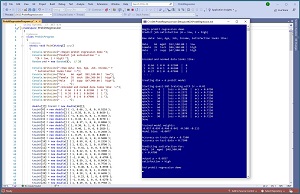 [Click on image for larger view.] Figure 1: Probit Regression Using C# in Action
A good way to see where this article is headed is to take a look at the screenshot of a demo program in Figure 1. The demo sets up 40 data items that represent employees. There are four predictor variables: sex (male = -1, female = +1), age (divided by 100), job-type (mgmt. = 1 0 0, supp = 0 1 0, tech = 0 0 1), and income (divided by $100,000). Each employee has a job satisfaction value encoded as 0 = low, 1 = high. The goal is to predict job satisfaction from the four predictor values.
The demo also sets up an 8-item test dataset to evaluate the model after training. The training and test datasets are completely artificial.
The demo program uses the 40-item training data and a modified form of stochastic gradient descent (SGD) to create a probit regression prediction model. After training, the model scores 75 percent accuracy on the training data (30 out of 40 correct), and also 75 percent accuracy on the test data (6 out of 8 correct).
The demo program concludes by making a prediction for a new, previously unseen data item where sex = male, age = 24, job-type = mgmt., income = $48,500. The output of the model is a p-value of 0.6837. Because the p-value is greater than 0.5 the prediction is job satisfaction = high. If the p-value had been less than 0.5 the prediction would have been job satisfaction = low.
This article assumes you have intermediate or better programming skill with the C# language but doesn't assume you know anything about probit regression. The complete demo code and the associated data are presented in this article. The source code and the data are also available in the accompanying download. All normal error checking has been removed to keep the main ideas as clear as possible.
Understanding Probit Regression
Suppose, as in the demo, you want to predict job satisfaction from sex, age, job-type, and income. The input values corresponding to (male, 24, mgmt, $48,500) are (x0, x1, x2, x3, x4, x5) = (-1, 0.24, 1, 0, 0, 0.485). Numeric values are normalized so that they're all between 0 and 1, Boolean values are minus-one plus-one encoded, and categorical values are one-hot encoded. There are several normalization and encoding alternatives, but the scheme used by the demo is simple and works well in practice.
Each input value has an associated numeric constant called a weight. There is an additional constant called a bias. For the demo problem, the model weights are (w0, w1, w2, w3, w4, w5) = (-0.057, 0.099, 0.460, 0.041, -0.508, -0.113) and the model bias is b = -0.0077.
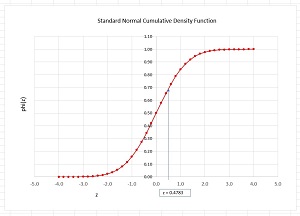 [Click on image for larger view.] Figure 2: The phi() Function
The first step is to compute a z-value as the sum of the products of the weights times the inputs, plus the bias:
z = (w0 * x0) +  (w1 * x1) +  (w2 * x2) +  (w3 * x3) +  (w4 * x4) +  (w5 * x5) +  b
  = (-0.057 * -1) + (0.099 * 0.24) + (0.460 * 1) + (0.041 * 0) + (-0.508 * 0) +
      (-0.113 * 0.485) + (-0.0077)
  = 0.0570 + 0.0238 + 0.4600 + 0.0000 + 0.0000 + (-0.0548) + (-0.0077)
  = 0.4783
The second step is to pass the computed z-value to the phi() function:
p = phi(0.4783)
  = 0.6837
The p-value result will be a value between 0.0 and 1.0 where a value less than 0.5 indicates a prediction of class 0 (low satisfaction in the demo) and p-value greater than 0.5 indicates a prediction of class 1 (high satisfaction). Therefore, for this example, the prediction is that the employee has high job satisfaction.
The phi() function is the cumulative density function (CDF) of the standard Normal distribution. For any input z-value, the phi() function returns the area under the Normal distribution from negative infinity to z. The graph in Figure 2 shows the phi() function where an input of z = 0.4783 returns p = 0.6837.
The two main challenges when creating a probit regression model are 1.) training the model to find the values of the weights and the bias, and 2.) writing code to implement the phi() function.
The Demo Program
The complete demo program, with a few minor edits to save space, is presented in Listing 1. To create the program, I launched Visual Studio and created a new C# .NET Core console application named ProbitRegression. I used Visual Studio 2022 (free Community Edition) with .NET Core 6.0, but the demo has no significant dependencies so any version of Visual Studio and .NET library will work fine. You can use the Visual Studio Code program too.
After the template code loaded, in the editor window I removed all unneeded namespace references, leaving just the reference to the top-level System namespace. In the Solution Explorer window, I right-clicked on file Program.cs, renamed it to the more descriptive ProbitProgram.cs, and allowed Visual Studio to automatically rename class Program to ProbitProgram.
Listing 1: Probit Regression Demo Code
using System;  // .NET 6.0
namespace ProbitRegression
{
  class ProbitProgram
  {
    static void Main(string[] args)
    {
      Console.WriteLine("Begin probit regression demo ");
      Console.WriteLine("Predict job satisfaction " +
        "(0 = low, 1 = high) ");
      Random rnd = new Random(0);  // 28

      Console.WriteLine("Raw data: Sex, Age, Job, Income," +
        " Satisfaction looks like: ");
      Console.WriteLine("Male    66  mgmt  $52,100.00 |  low");
      Console.WriteLine("Female  35  tech  $86,300.00 |  high");
      Console.WriteLine("Male    27  supp  $47,900.00 |  high");
      Console.WriteLine(" . . . ");
      Console.WriteLine("Encoded and normed data looks like: ");
      Console.WriteLine("-1  0.66  1 0 0  0.52100  |  0 ");
      Console.WriteLine(" 1  0.35  0 0 1  0.86300  |  1 ");
      Console.WriteLine("-1  0.27  0 1 0  0.47900  |  1 ");
      Console.WriteLine(" . . . ");

      double[][] trainX = new double[40][];
      trainX[0] = new double[] { -1, 0.66, 1, 0, 0, 0.5210 };
      trainX[1] = new double[] { 1, 0.35, 0, 0, 1, 0.8630 };
      trainX[2] = new double[] { -1, 0.24, 0, 0, 1, 0.4410 };
      trainX[3] = new double[] { 1, 0.43, 0, 1, 0, 0.5170 };
      trainX[4] = new double[] { -1, 0.37, 1, 0, 0, 0.8860 };
      trainX[5] = new double[] { 1, 0.30, 0, 1, 0, 0.8790 };
      trainX[6] = new double[] { 1, 0.40, 1, 0, 0, 0.2020 };
      trainX[7] = new double[] { -1, 0.58, 0, 0, 1, 0.2650 };
      trainX[8] = new double[] { 1, 0.27, 1, 0, 0, 0.8480 };
      trainX[9] = new double[] { -1, 0.33, 0, 1, 0, 0.5600 };
      trainX[10] = new double[] { 1, 0.59, 0, 0, 1, 0.2330 };
      trainX[11] = new double[] { 1, 0.52, 0, 1, 0, 0.8700 };
      trainX[12] = new double[] { -1, 0.41, 1, 0, 0, 0.5170 };
      trainX[13] = new double[] { 1, 0.22, 0, 1, 0, 0.3500 };
      trainX[14] = new double[] { 1, 0.61, 0, 1, 0, 0.2980 };
      trainX[15] = new double[] { -1, 0.46, 1, 0, 0, 0.6780 };
      trainX[16] = new double[] { 1, 0.59, 1, 0, 0, 0.8430 };
      trainX[17] = new double[] { 1, 0.28, 0, 0, 1, 0.7730 };
      trainX[18] = new double[] { -1, 0.46, 0, 1, 0, 0.8930 };
      trainX[19] = new double[] { 1, 0.48, 0, 0, 1, 0.2920 };
      trainX[20] = new double[] { 1, 0.28, 1, 0, 0, 0.6690 };
      trainX[21] = new double[] { -1, 0.23, 0, 1, 0, 0.8970 };
      trainX[22] = new double[] { -1, 0.60, 1, 0, 0, 0.6270 };
      trainX[23] = new double[] { 1, 0.29, 0, 1, 0, 0.7760 };
      trainX[24] = new double[] { -1, 0.24, 0, 0, 1, 0.8750 };
      trainX[25] = new double[] { 1, 0.51, 1, 0, 0, 0.4090 };
      trainX[26] = new double[] { 1, 0.22, 0, 1, 0, 0.8910 };
      trainX[27] = new double[] { -1, 0.19, 0, 0, 1, 0.5380 };
      trainX[28] = new double[] { 1, 0.25, 0, 1, 0, 0.9000 };
      trainX[29] = new double[] { 1, 0.44, 0, 0, 1, 0.8980 };
      trainX[30] = new double[] { -1, 0.35, 1, 0, 0, 0.5380 };
      trainX[31] = new double[] { -1, 0.29, 0, 1, 0, 0.7610 };
      trainX[32] = new double[] { 1, 0.25, 1, 0, 0, 0.3450 };
      trainX[33] = new double[] { 1, 0.66, 1, 0, 0, 0.2210 };
      trainX[34] = new double[] { -1, 0.43, 0, 0, 1, 0.7450 };
      trainX[35] = new double[] { 1, 0.42, 0, 1, 0, 0.8520 };
      trainX[36] = new double[] { -1, 0.44, 1, 0, 0, 0.6580 };
      trainX[37] = new double[] { 1, 0.42, 0, 1, 0, 0.6970 };
      trainX[38] = new double[] { 1, 0.56, 0, 0, 1, 0.3680 };
      trainX[39] = new double[] { -1, 0.38, 1, 0, 0, 0.2600 };

      int[] trainY = new int[40] { 0, 0, 0, 1, 1, 0, 0, 0, 0, 1,
        1, 0, 1, 0, 1, 1, 1, 0, 0, 0, 1, 1, 1, 1, 0, 1, 0, 0, 0,
        1, 1, 1, 1, 1, 0, 1, 0, 0, 0, 1 };

      double[][] testX = new double[8][];
      testX[0] = new double[] { 1, 0.36, 0, 0, 1, 0.8670 };
      testX[1] = new double[] { -1, 0.26, 0, 0, 1, 0.4310 };
      testX[2] = new double[] { 1, 0.42, 0, 1, 0, 0.5190 };
      testX[3] = new double[] { -1, 0.37, 1, 0, 0, 0.8260 };
      testX[4] = new double[] { 1, 0.31, 0, 1, 0, 0.8890 };
      testX[5] = new double[] { 1, 0.42, 1, 0, 0, 0.2040 };
      testX[6] = new double[] { -1, 0.57, 0, 0, 1, 0.2750 };
      testX[7] = new double[] { -1, 0.32, 0, 1, 0, 0.5500 };

      int[] testY = new int[8] { 0, 0, 1, 1, 0, 0, 0, 1 };

      Console.WriteLine("Creating dim = 6 probit model ");
      int dim = 6; // number predictors

      double[] wts = new double[dim];
      double lo = -0.01; double hi = 0.01;
      for (int i = 0; i < wts.Length; ++i)
        wts[i] = (hi - lo) * rnd.NextDouble() + lo;
      double bias = 0.0;

      Console.WriteLine("Starting quasi-SGD training " +
        "with lr = 0.01 ");
      int maxEpochs = 100;
      double lr = 0.01;

      int N = trainX.Length;  // number training items
      int[] indices = new int[N];
      for (int i = 0; i < N; ++i)
        indices[i] = i;

      for (int epoch = 0; epoch < maxEpochs; ++epoch)
      {
        Shuffle(indices, rnd);
        for (int i = 0; i < N; ++i)  // each data item
        {
          int ii = indices[i];
          double[] x = trainX[ii];  // inputs
          double y = trainY[ii];    // target 0 or 1
          double p = ComputeOutput(x, wts, bias);  // [0.0, 1.0]

          for (int j = 0; j < dim; ++j)  // each predictor weight
            wts[j] += lr * x[j] * (y - p) *
              p * (1 - p);  // o-t error => t-o update
          bias += lr * (y - p) * p * (1 - p);  // update bias
        }

        if (epoch % 10 == 0)
        {
          double mse = Error(trainX, trainY, wts, bias);
          double acc = Accuracy(trainX, trainY, wts, bias);
          Console.WriteLine("epoch = " +
            epoch.ToString().PadLeft(4) +
            "  |  loss = " + mse.ToString("F4") +
            "  |  acc = " + acc.ToString("F4"));
        }
      }
      Console.WriteLine("Done ");

      Console.WriteLine("Trained model weights: ");
      ShowVector(wts, 3, false);
      Console.WriteLine("Model bias: " + bias.ToString("F4"));

      double accTrain = Accuracy(trainX, trainY, wts, bias);
      Console.WriteLine("Accuracy on train data = " +
        accTrain.ToString("F4"));

      double accTest = Accuracy(testX, testY, wts, bias);
      Console.WriteLine("Accuracy on test data = " +
        accTest.ToString("F4"));

      Console.WriteLine("Predicting satisfaction for: ");
      Console.WriteLine("Male  24  mgmt  $48,500.00 ");
      double[] xx = new double[] { -1, 0.24, 1, 0, 0, 0.485 };
      double pp = ComputeOutput(xx, wts, bias, true);
      Console.WriteLine("output p = " + pp.ToString("F4"));
      if (pp < 0.5)
        Console.WriteLine("satisfaction = low");
      else
        Console.WriteLine("satisfaction = high");

      Console.WriteLine("End probit regression demo ");
      Console.ReadLine();
    } // Main

    static double Phi(double z)
    {
      // cumulative density of Standard Normal
      // erf is Abramowitz and Stegun 7.1.26

      if (z < -6.0)
        return 0.0;
      if (z > 6.0)
        return 1.0;

      double a0 = 0.3275911;
      double a1 = 0.254829592;
      double a2 = -0.284496736;
      double a3 = 1.421413741;
      double a4 = -1.453152027;
      double a5 = 1.061405429;

      int sign = 0;
      if (z < 0.0)
        sign = -1;
      else
        sign = 1;

      double x = Math.Abs(z) / Math.Sqrt(2.0);  // inefficient
      double t = 1.0 / (1.0 + a0 * x);
      double erf = 1.0 - (((((a5 * t + a4) * t) +
        a3) * t + a2) * t + a1) * t * Math.Exp(-x * x);
      return 0.5 * (1.0 + (sign * erf));
    }

    static double ComputeOutput(double[] x, double[] wts,
      double bias, bool showZ = false)
    {
      double z = 0.0;
      for (int i = 0; i < x.Length; ++i)
        z += x[i] * wts[i];
      z += bias;
      if (showZ == true)
        Console.WriteLine("z = " + z.ToString("F4"));
      return Phi(z);  // probit
      // return Sigmoid(z);  // logistic sigmoid
    }

    static double Error(double[][] dataX, int[] dataY,
      double[] wts, double bias)
    {
      double sum = 0.0;
      int N = dataX.Length;
      for (int i = 0; i < N; ++i)
      {
        double[] x = dataX[i];
        int y = dataY[i];  // target, 0 or 1
        double p = ComputeOutput(x, wts, bias);
        sum += (p - y) * (p - y); // E = (o-t)^2 form
      }
      return sum / N; ;
    }

    static double Accuracy(double[][] dataX, int[] dataY,
      double[] wts, double bias)
    {
      int numCorrect = 0; int numWrong = 0;
      int N = dataX.Length;
      for (int i = 0; i < N; ++i)
      {
        double[] x = dataX[i];
        int y = dataY[i];  // actual, 0 or 1
        double p = ComputeOutput(x, wts, bias);
        if (y == 0 && p < 0.5 || y == 1 && p >= 0.5)
          ++numCorrect;
        else
          ++numWrong;
      }
      return (1.0 * numCorrect) / (numCorrect + numWrong);
    }

    static double AccuracyVerbose(double[][] dataX,
      int[] dataY, double[] wts, double bias)
    {
      int numCorrect = 0; int numWrong = 0;
      int N = dataX.Length;
      for (int i = 0; i < N; ++i)
      {
        Console.WriteLine("=========");
        double[] x = dataX[i];
        int y = dataY[i];  // actual, 0 or 1
        double p = ComputeOutput(x, wts, bias);

        Console.WriteLine(i);
        ShowVector(x, 1, false);
        Console.WriteLine("target = " + y);
        Console.WriteLine("computed = " + p.ToString("f4"));

        if (y == 0 && p < 0.5 || y == 1 && p >= 0.5)
        {
          Console.WriteLine("correct ");
          ++numCorrect;
        }
        else
        {
          Console.WriteLine("wrong ");
          ++numWrong;
        }
        Console.WriteLine("=========");
        Console.ReadLine();
      }
      return (1.0 * numCorrect) / (numCorrect + numWrong);
    }

    static void Shuffle(int[] arr, Random rnd)
    {
      int n = arr.Length;
      for (int i = 0; i < n; ++i)
      {
        int ri = rnd.Next(i, n);
        int tmp = arr[ri];
        arr[ri] = arr[i];
        arr[i] = tmp;
      }
    }

    static void ShowVector(double[] vector, int decs,
      bool newLine)
    {
      for (int i = 0; i < vector.Length; ++i)
        Console.Write(vector[i].ToString("F" + decs) + " ");
      Console.WriteLine("");
      if (newLine == true)
        Console.WriteLine("");
    }

  } // Program
} // ns
The demo program hard-codes the training and test input x-data as array-of-arrays style matrices, and the target y-data as int[] vectors. In a non-demo scenario, you will probably want to store data in a text file and write a helper function to read the data into the matrices and vectors.
All the control logic is in the Main() method. The probit model is defined as an array named wts and a variable named bias. An alternative design is to place the weights and bias in a class along the lines of:
public class ProbitModel
{
  public double[] wts;
  public double bias;
  public ProbitModel(int dim)
  {
    this.wts = new double[dim];
    this.bias = 0.0;
  }
}
Defining a probit model as two separate variables is simpler than using a class but a bit less flexible.
Implementing the Phi() Function
There is no simple way to explicitly define the phi() function but there are several ways to estimate the phi() function. One common way to define phi() is to use a helper function called the erf() function. The code in Listing 2 shows one approach.
Listing 2: The Phi() Function
static double Phi(double z)
{
  if (z < -6.0)
    return 0.0;
  if (z > 6.0)
    return 1.0;

  double a0 = 0.3275911;
  double a1 = 0.254829592;
  double a2 = -0.284496736;
  double a3 = 1.421413741;
  double a4 = -1.453152027;
  double a5 = 1.061405429;

  int sign = 0;
  if (z < 0.0)
    sign = -1;
  else
    sign = 1;

  double x = Math.Abs(z) / Math.Sqrt(2.0);
  double t = 1.0 / (1.0 + a0 * x);
  double erf = 1.0 - (((((a5 * t + a4) * t) +
    a3) * t + a2) * t + a1) * t * Math.Exp(-x * x);
  return 0.5 * (1.0 + (sign * erf));
}
The function begins by short-circuiting for input values of less than -6.0 or greater than +6.0 because the phi() function is very close to 0.0 or 1.0 for those inputs. The erf ("error function") value is estimating using what is called equation A&S 7.1.26. The Wikipedia entry on "Error Function" presents several alternative ways to estimate the erf() function.
To recap, probit regression uses the phi() function which is an area under than Standard Normal distribution. To estimate phi() you can use a special erf() function, and to estimate erf() you can use math equation A&S 7.1.26.
The implementation of the phi() function is not at all obvious. But you can think of phi() as a black box that accepts any input and returns a value between 0.0 and 1.0. You will not need to modify the implementation of the phi() function except in rare cases.
Training the Model
Training a probit model is the process of using training data with known input and correct output values to find good values for the model weights and the bias. There are several ways to train a probit model including stochastic gradient descent (SGD), L-BFGS optimization, iterated Newton-Raphson, and particle swarm optimization. The demo program uses a modified form of SGD.
In high-level pseudo-code:
loop several times
    scramble order of training data
    for-each training data item
      get inputs x
      get target y (0 or 1)
      compute output p using curr wts and bias
      adjust all wts and bias so output is closer to target
    end-for
  end-loop
The key statements that update each weight and the bias are:
for (int j = 0; j < dim; ++j)  // each weight
  wts[j] += lr * x[j] * (y - p) * p * (1 - p);

bias += lr * (y - p) * p * (1 - p);  // update bias
Suppose that for the current input values in x[], the correct target value is y = 1 and the computed output value is p = 0.65. You want to adjust the weights so that the computed output will increase and get closer to the target. The difference between target and computed is (y - p) = (1 - 0.65) = +0.35. You could use this difference and add it to all weights and the bias. However, that approach is too aggressive so you scale back the difference by multiplying by a constant called the learning rate (lr). In the demo, the learning rate is set to 0.01. A good value of the learning rate must be found by trial and error. Common values are 0.10, 0.01, and 0.005.
The update value also includes an x[j] term which is the associated input for the weight. This is necessary to take into account the sign of the input to keep the weight update in the correct direction.
The update value also has a term of p * (1 - p). If computed p = 0.65 then (1 - p) = 0.35 and p * (1 - p) = 0.65 * 0.35 = 0.2275. The p * (1 - p) term will be largest when computed p = 0.5 which is when the output is most ambiguous. When p is close to 0.0 or 1.0, the output is less ambiguous and the p * (1 - p) term will be small.
Wrapping Up
Probit regression is not used as often as logistic regression because the two techniques usually give similar results and logistic regression is a bit easier to implement than probit regression. Both probit regression and logistic regression are relatively crude techniques for binary classification. The biggest disadvantage of both techniques is that they can only work well with data that is close to linearly separable. This means you can hypothetically draw a line or hyperplane through the data so that class 0 data items are on one side and class 1 items are on the other.
For complex data, a neural binary classifier usually works better than probit regression or logistic regression. However, a neural classifier usually requires large amounts of training data, and is significantly more difficult to implement than probit regression. When presented with a binary classification problem, a common strategy is to try probit or logistic regression first. If the resulting model is not satisfactory then you can try a neural model and use the probit model results as a baseline result for comparison.