The Data Science Lab
How to Do Machine Learning Evolutionary Optimization Using C#
Resident data scientist Dr. James McCaffrey of Microsoft Research turns his attention to evolutionary optimization, using a full code download, screenshots and graphics to explain this machine learning technique used to train many types of models by modeling the biological processes of natural selection, evolution, and mutation.
Evolutionary optimization is a technique that can be used to train many types of machine learning models. Evolutionary optimization loosely models the biological processes of natural selection, evolution, and mutation.
Although it's possible to learn about evolutionary optimization by seeing how it works with an abstract problem, in my opinion it's better to start with a concrete example. In this article I demonstrate how to use evolutionary optimization to train a logistic regression model. Along the way, I'll explain how to adapt the example to other types of machine learning models.
Logistic regression classification is arguably the most fundamental machine learning technique. Logistic regression can be used for binary classification, for example predicting if a person is male or female based on predictors such as age, height, weight, and so on.
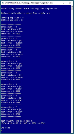
Take a look at the demo program in the screenshot in Figure 1. The goal of the demo is to predict the authenticity of a banknote (think dollar bill or euro) based on four predictor values (variance, skewness, kurtosis, entropy). The demo sets up a population of six possible solutions then uses eight generations of evolutionary optimization to find successively better solutions.
Behind the scenes, the demo program sets up a training dataset of 40 items. In the first generation, the best solution is at [5] in the population and that solution has prediction accuracy of 60 percent (24 correct, 16 wrong) and error of 0.2266. After eight generations of evolution, a solution is found that scores 87.50 percent accuracy (35 correct, 5 wrong) with 0.0956 error.
The demo concludes by displaying the four weights and one bias values for a logistic regression model: (-0.9435, -0.8266, -0.2915, -0.6601, -0.0369). In a non-demo scenario, these values would be used to make a prediction, or be saved to file for later use.
 [Click on image for larger view.] Figure 1: Evolutionary Optimization for Logistic Regression Demo
This article assumes you have intermediate or better skill with C# and a basic understanding of logistic regression but doesn’t assume you know anything about evolutionary optimization. The code for demo program is a bit too long to present in its entirety in this article but the complete code is available in the associated file download.
Understanding the Data
The demo program uses a small 40-item subset of a well-known benchmark collection of data called the Banknote Authenticity Dataset. The full dataset has 1,372 items, with 762 authentic and 610 forgery items. You can find the complete dataset in many places on the Internet.
The raw data looks like:
3.6216, 8.6661, -2.8073, -0.44699, 0
4.5459, 8.1674, -2.4586, -1.4621, 0
. . .
-3.5637, -8.3827, 12.393, -1.2823, 1
-2.5419, -0.65804, 2.6842, 1.1952, 1
Each line represents a banknote. The first four values on each line are characteristics of a digital image of the banknote: variance, skewness, kurtosis, and entropy. The fifth value on a line is 0 for an authentic note and 1 for a forgery. The demo program uses only the first 20 authentic notes and the first 20 forgeries of the full dataset.
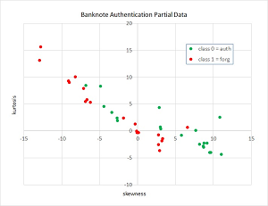
Because the data has four dimensions, it's not possible to display the data in a two-dimensional graph. However, you can get an idea of what the data is like by taking a look at a graph of partial data shown in Figure 2.
 [Click on image for larger view.] Figure 2: Graph of the Banknote Data
The graph plots just the skewness and kurtosis of the 40 data items used in the demo. The graph shows that classifying a banknote as authentic or forgery is a fairly difficult problem.
Quick Summary of Logistic Regression Classification
Logistic regression classification is relatively simple. For a dataset with n predictor variables, there will be n weights plus one special weight called a bias. Weights and biases are just numeric constants with values like -1.2345 and 0.9876. To make a prediction, you sum the products of each predictor value and its associated weight and then add the bias. The sum is often given the symbol z. Then you take the logistic sigmoid of z to get a p-value. If the p-value is less than 0.5 then the prediction is class 0 and if the p-value is greater than or equal to 0.5 then the prediction is class 1.
For example, suppose you have a dataset with three predictor variables and suppose that the three associated weight values are (0.20, -0.40, 0.30) and the bias value is 1.10. If an item to predict has values (5.0, 6.0, 7.0) then:
z = (0.20 * 5.0) + (-0.40 * 6.0) + (0.30 * 7.0) + 1.10
   = 1.80
p = 1.0 / (1.0 + exp(-1.80))
   = 0.8581
Because p is greater than or equal to 0.5 the predicted class is 1.
The function f(x) = 1.0 / (1.0 + exp(-x)) is called the logistic sigmoid function. The function exp(x) is Euler's number, approximately 2.718, raised to the power of x.
Determining the values of the weights and bias is called training the model. In addition to evolutionary optimization, there are many other techniques that can be used to train a logistic regression model. Three common training techniques for logistic regression are stochastic gradient descent (SGD), iterated Newton-Raphson, and L-BFGS optimization.
Understanding Evolutionary Optimization
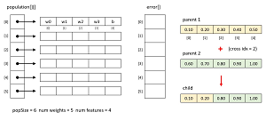
The images in Figure 3 illustrate the key ideas of evolutionary optimization. Because the banknote data has four predictors/features, a logistic regression model solution will have five values – four weights and one bias. Evolutionary optimization creates a population of solutions. The demo uses a population size of six. Each solution has an associated error. The demo uses mean squared error between computed outputs (values between 0.0 and 1.0) and correct outputs (0 or 1).
 [Click on image for larger view.] Figure 3: Evolutionary Optimization
Evolutionary optimization is an iterative process. In pseudo-code:
create a population of (random) solutions
loop maxGen times
  pick two good solutions
  use good solutions to create a child solution
  mutate child slightly
  replace a bad solution with child solution
  create a random solution
  replace a bad solution with the random solution
end-loop
return best solution found
If parent1 and parent2 are two good (low error) solutions in the population, to create a child solution you start by generating a random crossover index. Then the child receives the values from the left part of parent1 and the right part of parent2. An alternative approach is to create an additional second child with the right part of parent1 and the left part of parent2.
Mutation is an important part of evolutionary optimization. The approach used in the demo program is:
loop each cell of child solution
  generate a random probability p
  if p is small give cell a new random value
end-loop
A key task when using evolutionary optimization is selecting relatively good and bad solutions so that you can use good solutions to generate a new child solution, and you can replace a bad solution with a child solution or a new random solution. The demo program uses a technique called tournament selection. To select a good solution:
set alpha = value between 0 percent and 100 percent
select a random alpha percent subset of population indices
return best index (lowest error) of subset
Suppose, as in the demo, the population size is six and so the indices of the population are (0, 1, 2, 3, 4, 5). And suppose alpha is set to 0.50. This means that a random 0.50 * 6 = 3 indices are selected, for example, (4, 0, 2). From these three, the solution with the lowest error is selected.
The alpha parameter is called the selection pressure. The larger alpha is, the more likely you are to get the absolute best solution in the population. A good value for alpha is problem-dependent and must be determined by trial and error, but 0.80 is a reasonable value to start.
To select a random subset of size n from all population indices, the demo program starts with all indices (0, 1, 2, 3, 4, 5) then shuffles the indices using the Fisher-Yates mini-algorithm, giving for example (3, 5, 0, 1, 4, 2), and then returns the first n indices (3, 5, 0). Simple and effective.
Selecting the index of a relatively bad solution is exactly like selecting a good solution except that after sampling you return the index of the solution that has the highest error.
The Demo Program
To create the demo program, I launched Visual Studio 2019. I used the Community (free) edition but any relatively recent version of Visual Studio will work fine. From the main Visual Studio start window I selected the "Create a new project" option. Next, I selected C# from the Language dropdown control and Console from the Project Type dropdown, and then picked the "Console App (.NET Core)" item.
The code presented in this article will run as a .NET Core console application or as a .NET Framework application. Many of the newer Microsoft technologies, such as the ML.NET code library, specifically target .NET Core so it makes sense to develop most new C# machine learning code in that environment.
I entered "LogisticEvo" as the Project Name, specified C:\VSM on my local machine as the Location (you can use any convenient directory), and checked the "Place solution and project in the same directory" box.
After the template code loaded into Visual Studio, at the top of the editor window I removed all using statements to unneeded namespaces, leaving just the reference to the top level System namespace. The demo needs no other assemblies and uses no external code libraries.
In the Solution Explorer window, I renamed file Program.cs to the more descriptive LogisticEvoProgram.cs and then in the editor window I renamed class Program to class LogisticEvoProgram to match the file name. The structure of the demo program, with a few minor edits to save space, is shown in Listing 1.
Listing 1. Evolutionary Optimization Demo Program Structure
using System;
namespace LogisticEvo
{
  class LogisticEvoProgram
  {
    static void Main(string[] args)
    {
      Console.WriteLine("Evolutionary optimization");
      Console.WriteLine("Banknote authenticity");

      // Banknote Authentication subset
      double[][] trainX = new double[40][];
      trainX[0] = new double[] { 3.6216, 8.6661,
        -2.8073, -0.44699 };
      trainX[1] = new double[] { 4.5459, 8.1674,
        -2.4586, -1.4621 };
      . . .
      trainX[38] = new double[] { -3.5801, -12.9309,
        13.1779, -2.5677 };
      trainX[39] = new double[] { -1.8219, -6.8824,
        5.4681, 0.057313 };

      int[] trainY = new int[] {
        0, 0, 0, 0, 0, 0, 0, 0, 0, 0,
        0, 0, 0, 0, 0, 0, 0, 0, 0, 0,
        1, 1, 1, 1, 1, 1, 1, 1, 1, 1,
        1, 1, 1, 1, 1, 1, 1, 1, 1, 1 };

      int popSize = 6;
      int maxGen = 8;
      double alpha = 0.40;    // selection pressure
      double sigma = 0.80;  // selection (child)
      double omega = 0.50;  // selection (new soln)
      double mRate = 0.05;  // mutation rate

      double[] wts = Train(trainX, trainY, popSize,
       maxGen, alpha, sigma, omega, mRate, seed: 3);

      Console.WriteLine("Best weights found:");
      ShowVector(wts);

      Console.WriteLine("End demo ");
      Console.ReadLine();
    } // Main

    static double[] Train(double[][] trainX,
      int[] trainY, int popSize, int maxGen,
      double alpha, double sigma, double omega,
      double mRate, int seed) { . . }

    static double[] MakeSolution(int nw,
      Random rnd) { . . }

    static double[][] MakePopulation(int popSize,
      int nw, Random rnd) { . . }

    static double[] MakeChild(double[][] pop,
      int[] parents, Random rnd) { . . }

    static void Mutate(double[] child,
      double mRate, Random rnd) { . . }

    static int BestSolution(double[] errors) { . . }

    static int SelectGood(double[] errors,
      double pct, Random rnd) { . . }

    static int[] SelectTwo(double[] errors,
      double pct, Random rnd) { . . }

    static int SelectBad(double[] errors,
      double pct, Random rnd) { . . }

    static void Shuffle(int[] vec,
      Random rnd) { . . }

    static double ComputeOutput(double[] x,
      double[] wts) { . . }

    static double LogSig(double x) { . . }

    static double Accuracy(double[][] dataX,
      int[] dataY, double[] wts) { . . }

    static double Error(double[][] dataX,
      int[] dataY, double[] wts) { . . }

    static void ShowVector(double[] v) { . . }
  }
} // ns
The program isn't as complicated as it might appear because most of the functions are relatively small and simple helpers. All of the program logic is contained in the Main() method. The demo uses a static method approach rather than an OOP approach for simplicity. All normal error checking has been removed to keep the main ideas as clear as possible.
The demo begins by setting up the 40-item training data:
double[][] trainX = new double[40][];
trainX[0] = new double[] { 3.6216, 8.6661,
  -2.8073, -0.44699 };
. .
trainX[39] = new double[] { -1.8219, -6.8824,
  5.4681, 0.057313 };
int[] trainY = new int[40] {
  0, 0, . . 1 };
In a non-demo scenario you'd likely want to store your training data as a text file and then you'd read the training data into memory using helper functions along the lines of:
double[][] trainX = MatLoad("..\\trainData.txt",
  new int[] { 0, 1, 2, 3 }, ",");
int[] trainY = VecLoad("..\\trainData.txt", 4, ",");
Because of the way logistic regression classification output is computed, it's almost always a good idea to normalize your training data so that small predictor values (such as an age of 35) aren't overwhelmed by large predictor values (such as an annual income of 65,000.00). The three most common normalization techniques are min-max normalization, z-score normalization and order of magnitude normalization. Because the banknote predictor values all are roughly within the same magnitude, the demo does not normalize the training data.
In many scenarios you'd want to set aside some of your source data as a test dataset. After training you'd compute the prediction accuracy of the model on the held-out dataset. This accuracy metric would be a rough estimate of the accuracy you could expect on new, previously unseen data.
After setting up the training data, the demo program trains the model using these statements:
int popSize = 6;
int maxGen = 8;
double alpha = 0.40;  // selection pressure
double sigma = 0.80;  // selection (child)
double omega = 0.50;  // selection (new soln)
double mRate = 0.05;  // mutation rate

double[] wts = Train(trainX, trainY, popSize,
  maxGen, alpha, sigma, omega, mRate, seed: 3);
The population size and maximum number of generations to evolve are hyperparameters that must be determined by trial and error. The values of hyperparameters alpha, sigma and omega control selection pressure for picking good parents to breed, picking a bad solution for replacement by a child, and picking a bad solution for replacement by a new random solution.
The mutation rate controls how many cells in a newly created child solution will be randomly mutated. In my experience, of the six training hyperparameters, evolutionary optimization is more sensitive to the mutation rate than the other parameters.
The Train() function accepts a seed value which is used to create a local Random object. The seed value in the demo, 3, was used only because it gave a representative result.
Implementation Details
The demo program defines a MakeSolution() function like so:
static double[] MakeSolution(int nw, Random rnd)
{
  double lo = -1.0; double hi = 1.0;
  double[] soln = new double[nw];
  for (int i = 0; i < nw; ++i)
    soln[i] = (hi - lo) * rnd.NextDouble() + lo;
  return soln;
}
The function creates a vector with a size equal to the number of weights (including the bias) needed for a logistic regression problem. Each cell of the vector holds a random value in the range [-1.0, +1.0] which is a problem-dependent hyperparameter.
The code to create a child solution from two parent solutions is:
static double[] MakeChild(double[][] pop,
  int[] parents, Random rnd)
{
  int nw = pop[0].Length;  // num wts including bias
  int idx = rnd.Next(1, nw);  // crossover
  double[] child = new double[nw];
  for (int j = 0; j < idx; ++j)
    child[j] = pop[parents[0]][j];  // left
  for (int j = idx; j < nw; ++j)
    child[j] = pop[parents[1]][j];  // right
   return child;
}
The child contains the values of parent1 from index [0] up to but not including a randomly generated [index], and from [index] to the last cell of parent2.
The code to mutate a newly created child solution is defined in function Mutate() and is:
static void Mutate(double[] child, double mRate,
  Random rnd)
{
  double lo = -1.0; double hi = 1.0;
  for (int i = 0; i < child.Length; ++i) {
    double p = rnd.NextDouble();
    if (p < mRate)  // rarely
      child[i] = (hi - lo) * rnd.NextDouble() + lo;
  }
  return;
}
The function traverses a child solution and modifies each cell independently with probability mRate. Because the function modifies its child parameter directly, I use an explicit return statement as a form of documentation.
Wrapping Up
Evolutionary optimization is a meta-heuristic, meaning the technique is a set of general guidelines rather than a rigid algorithm. This means you have many design choices, such as creating two children at a time instead of one, using two crossover points instead of one for mutation, and so on. Based on my experience with evolutionary optimization, simplicity is a better approach than sophistication.
Evolutionary optimization can be used to train any kind of machine learning model that has a well-defined solution and a way to compute error for a solution. In particular, evolutionary optimization can be used to train a neural network or any kernel-based model.
The main advantage of evolutionary optimization is that, unlike many machine learning training algorithms, it does not require a Calculus gradient. The main disadvantage of evolutionary optimization is that it usually requires far more processing time than gradient-based techniques.
Evolutionary optimization has existed for many years but there's been renewed interest in the technique recently. Even though I have no solid survey data, there seems to be a growing sense among researchers that regular deep neural networks, which rely on Calculus gradients, are reaching the limits of their capabilities. New approaches, such as neuromorphic computing, are gaining increased attention. Many of these newer approaches cannot use gradients and so evolutionary optimization is one possible option for training.