The Data Science Lab
Autoencoder Anomaly Detection Using PyTorch
Dr. James McCaffrey of Microsoft Research provides full code and step-by-step examples of anomaly detection, used to find items in a dataset that are different from the majority for tasks like detecting credit card fraud.
Anomaly detection is the process of finding items in a dataset that are different in some way from the majority of the items. For example, you could examine a dataset of credit card transactions to find anomalous items that might indicate a fraudulent transaction. This article explains how to use a PyTorch neural autoencoder to find anomalies in a dataset.
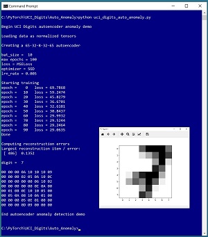
A good way to see where this article is headed is to take a look at the screenshot of a demo program in Figure 1. The demo analyzes a dataset of 3,823 images of handwritten digits where each image is 8 by 8 pixels. The demo program presented in this article uses image data, but the autoencoder anomaly detection technique can work with any type of data.
The demo begins by creating a Dataset object that stores the images in memory. Next, the demo creates a 65-32-8-32-65 neural autoencoder. An autoencoder learns to predict its input. Therefore, the autoencoder input and output both have 65 values -- 64 pixel grayscale values (0 to 16) plus a label (0 to 9). Notice that the demo program analyzes both the predictors (pixel values) and the dataset labels (digits). Depending upon your particular anomaly detection scenario, you might not include the labels.
The demo sets up training parameters for the batch size (10), number of epochs to train (100), loss function (mean squared error), optimization algorithm (stochastic gradient descent) and learning rate (0.005). After training the autoencoder, the demo scans the dataset and computes the reconstruction error for each data item. The data item that has the largest error is item [486] with error = 0.1352. The demo concludes by displaying that anomalous item, which is a "7" digit.
 [Click on image for larger view.] Figure 1: Autoencoder Anomaly Detection in Action
This article assumes you have an intermediate or better familiarity with a C-family programming language, preferably Python, but doesn't assume you know very much about PyTorch. The complete source code for the demo program is presented in this article. The source code is also available in the accompanying file download. All normal error checking code has been omitted to keep the main ideas as clear as possible.
To run the demo program, you must have Python and PyTorch installed on your machine. The demo programs were developed on Windows 10 using the Anaconda 2020.02 64-bit distribution (which contains Python 3.7.6) and PyTorch version 1.8.0 for CPU installed via pip. Installation is not trivial. You can find detailed step-by-step installation instructions for this configuration in my blog post.
The UCI Digits Dataset
The UCI Digits dataset can be found here. There is a 3,823-item file named optdigits.tra (intended for training) and a 1,797-item file named optdigits.tes (for testing). I downloaded the files and renamed them to optdigits_train_3823.txt and optdigits_test_1797.txt. Each file is a simple, comma-delimited text file. Each line represents an 8 by 8 handwritten digit from "0" to "9."
The UCI Digits dataset resembles the well-known MNIST dataset. MNIST has 60,000 training and 10,000 test image. Each image is 28 by 28 = 784 pixels, and the source MNIST files are stored in a proprietary binary format. The UCI digits dataset is much easier to work with.
The UCI Digits data looks like:
0,1,6,16,12, . . . 1,0,0,13,0
2,7,8,11,15, . . . 16,0,7,4,1
. . .
The first 64 values on each line are the image pixel values. Each pixel is a grayscale value between 0 and 16. The last value on each line is the digit/label. There are about 380 of each digit in the training file and about 180 of each digit in the test file, but the digits are not evenly distributed. The counts of each "0" though "9" digit are:
optdigits_train_3823.txt:
[376, 389, 380, 389, 387, 376, 377, 387, 380, 382]

optdigits_test_1797.txt:
[178, 182, 177, 183, 181, 182, 181, 179, 174, 180]
The 10 images in Figure 2 are representative digits. With only 64 pixels, each image is quite crude when displayed visually.
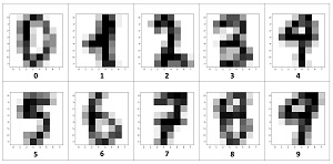 [Click on image for larger view.] Figure 2: Examples of UCI Digits Data Displayed Visually
The demo program defines a PyTorch Dataset class to load the data in memory. See Listing 1.
Listing 1: A Dataset Class for the UCI Digits Data
import torch as T
import numpy as np

class UCI_Digits_Dataset(T.utils.data.Dataset):
  # 8,12,0,16, . . 15,7
  # 64 pixel values [0-16], digit [0-9]

  def __init__(self, src_file, n_rows=None):
    all_xy = np.loadtxt(src_file, max_rows=n_rows,
      usecols=range(0,65), delimiter=",", comments="#",
      dtype=np.float32)
    self.xy_data = T.tensor(all_xy, dtype=T.float32).to(device)
    self.xy_data[:, 0:64] /= 16.0   # normalize pixels
    self.xy_data[:, 64] /= 9.0      # normalize digit/label

  def __len__(self):
    return len(self.xy_data)

  def __getitem__(self, idx):
    xy = self.xy_data[idx]
    return xy
The class loads a file of UCI digits data into memory as a two-dimensional array using the NumPy loadtxt() function. Alternatives loading functions include the NumPy genfromtxt() or fromfile() functions, or the Pandas read_csv() function. After converting the NumPy array to a PyTorch tensor array, the pixel values in columns [0] to [63] are normalized by dividing by 16, and the label values in column [64] are normalized by dividing by 9. The resulting pixel and label values are all between 0.0 and 1.0.
In most scenarios, the __getitem__() method returns a Python tuple with predictors and labels. But for an autoencoder, each data item acts as both the input and the target to predict.
The Dataset can be used with code like this:
fn = ".\\Data\\optdigits_train_3823.txt"
my_ds = UCI_Digits_Dataset(fn)
my_ldr = T.utils.data.DataLoader(my_ds, \
  batch_size=10, shuffle=True)
for (b_ix, batch) in enumerate(my_ldr):
  # b_ix is the batch index
  # batch item has 65 values between 0 and 1
. . .
The Dataset object is passed to a built-in PyTorch DataLoader object. The DataLoader object serves up the data in batches of a specified size, in a random order on each pass through the Dataset.
The design pattern presented here will work for most autoencoder anomaly detection scenarios. If your raw data contains a categorical variable, such as "color" with possible values "red", "blue" or "green", you can one-hot encode the data: "red" = (1, 0, 0), "blue" = (0, 1, 0), "green" = (0, 0, 1). If your source data is too large to load into memory, you'll have to write a custom data loader that buffers the data. I describe how to create streaming data loaders in a previous article; you can find it here .
Autoencoders
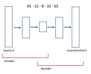
An autoencoder is a neural network that predicts its own input. The diagram in Figure 3 shows the architecture of the 65-32-8-32-65 autoencoder used in the demo program. An input image x, with 65 values between 0 and 1 is fed to the autoencoder. A neural layer transforms the 65-values tensor down to 32 values. The next layer produces a core tensor with 8 values. The core 8 values generate 32 values, which in turn generate 65 values. The size of the first and last layers of an autoencoder are determined by the problem data, but the number of interior hidden layers, and the number of nodes in each hidden layer, are hyperparameters that must be determined by trial and error guided by experience.
 [Click on image for larger view.] Figure 3: Autoencoder Architecture for the UCI Digits Dataset
The idea is that the first part of the autoencoder finds the fundamental information contained in the input image, stripping away noise and random error. The second part of the autoencoder generates a cleaned version of the input. The first part of an autoencoder is called the encoder component, and the second part is called the decoder.
To use an autoencoder for anomaly detection, you compare the reconstructed version of an image with its source input. If the reconstructed version of an image differs greatly from its input, the image is anomalous in some way.
The definition of the demo program autoencoder is presented in Listing 2. There are many design alternatives. The __init__() method defines four fully-connected ("fc") layers. You might want to parameterize __init__() to accept the layer sizes instead of hard-coding them as the demo does. The class uses default initialization for weights and biases. Weight and bias initialization is a surprisingly complex topic. You might want to explicitly initialize weights using the T.nn.init.uniform_() function. I sometimes get significantly better results using explicit weight initialization.
Listing 2: Autoencoder Definition for UCI Digits Dataset
class Autoencoder(T.nn.Module):  # 65-32-8-32-65
  def __init__(self):
    super(Autoencoder, self).__init__()
    self.fc1 = T.nn.Linear(65, 32)
    self.fc2 = T.nn.Linear(32, 8)
    self.fc3 = T.nn.Linear(8, 32)
    self.fc4 = T.nn.Linear(32, 65)

  def encode(self, x):  # 65-32-8
    z = T.tanh(self.fc1(x))
    z = T.tanh(self.fc2(z))  # latent in [-1,+1]
    return z

  def decode(self, x):  # 8-32-65
    z = T.tanh(self.fc3(x))
    z = T.sigmoid(self.fc4(z))  # [0.0, 1.0]
    return z

  def forward(self, x):  # 65-32-8-32-65
    z = self.encode(x)
    z = self.decode(z)
    return z  # in [0.0, 1.0]
The Autoencoder defines explicit encode() and decode() methods, and then defines the forward() method using encode() and decode(). Because an autoencoder for anomaly detection often doesn't directly use the values in the interior core layer, it's possible to eliminate encode() and decode() and define the forward() method directly:
def forward(self, x):
  z = T.tanh(self.fc1(x))
  z = T.tanh(self.fc2(z))  # latent in [-1,+1]
  z = T.tanh(self.fc3(z))
  z = T.sigmoid(self.fc4(z))  # [0.0, 1.0]
  return z
Using this approach, the first part of forward() acts as the encoder component and the second part acts as the decoder.
The demo program uses tanh() activation on all layers except the final output layer, where sigmoid() is used because the output values must be in range [0.0, 1.0] to match the input values. Many of the autoencoder examples I see online use relu() activation for interior layers. The relu() function was designed for use with very deep neural architectures. For autoencoders, which are usually relatively shallow, I often, but not always, get better results with tanh() activation.
The Overall Program Structure
The overall structure of the PyTorch autoencoder anomaly detection demo program, with a few minor edits to save space, is shown in Listing 3. I prefer to indent my Python programs using two spaces rather than the more common four spaces.
Listing 3: The Structure of the Autoencoder Anomaly Program
# uci_digits_auto_anomaly.py

# autoencoder reconstruction error anomaly detection
# uses an encoder-decoder architecture
# PyTorch 1.8.0-CPU Anaconda3-2020.02  Python 3.7.6
# Windows 10

import numpy as np
import matplotlib.pyplot as plt
import torch as T

device = T.device("cpu")

# -----------------------------------------------------------

class UCI_Digits_Dataset(T.utils.data.Dataset): . . .

class Autoencoder(T.nn.Module): . . .

def display_digit(ds, idx, save=False): . . .

def train(ae, ds, bs, me, le, lr): . . .

def make_err_list(model, ds): . . .

# -----------------------------------------------------------

def main():
  # 0. get started
  # 1. create Dataset object
  # 2. create autoencoder net
  # 3. train autoencoder model
  # 4. compute and store reconstruction errors
  # 5. show most anomalous data item

  print("End autoencoder anomaly detection demo ")

# -----------------------------------------------------------

if __name__ == "__main__":
  main()
It's important to document the versions of Python and PyTorch being used because both systems are under continuous development. Dealing with versioning incompatibilities is a significant headache when working with PyTorch and is something you should not underestimate.
I prefer to use "T" as the top-level alias for the torch package. Most of my colleagues don't use a top-level alias and spell out "torch" many times per program. Also, I use the full form of submodules rather than supplying aliases such as "import torch.nn.functional as functional." In my opinion, using the full form is easier to understand and less error-prone than using many aliases.
The demo program defines a program-scope CPU device object. I usually develop my PyTorch programs on a desktop CPU machine. After I get that version working, converting to a CUDA GPU system only requires changing the global device object to T.device("cuda") plus a minor amount of debugging.
The demo program defines three helper methods: display_digit(), train() and make_err_list(). All of the rest of the program control logic is contained in a main() function. Using helper functions makes the code a bit more difficult to understand, but allows you to manage and modify the code more easily.
The main function begins with:
def main():
  # 0. get started
  print("\nBegin UCI Digits autoencoder anomaly demo ")
  T.manual_seed(1)
  np.random.seed(1)

  # 1. create Dataset object
  print("Loading data as normalized tensors ")
  fn = ".\\Data\\optdigits_train_3823.txt"
  data_ds = UCI_Digits_Dataset(fn)  # all rows
  . . .
The demo program sets the NumPy and PyTorch random number generator seed values so that program runs will be reproducible. The seed value of 1 is arbitrary. The Dataset assumes that the source file is in a subdirectory named Data. The program continues with:
  # 2. create autoencoder net
  print("Creating a 65-32-8-32-65 autoencoder ")
  autoenc = Autoencoder().to(device)
  autoenc.train()   # set mode
The autoenc object is set into training mode. Technically, this is not necessary because train() mode is the default, but in my opinion it's good practice to explicitly set the mode. Because train() mode works by reference, it's not necessary to write autoenc = autoenc.train(). Next, the demo program trains the network using a program-defined train() function with these statements:
  # 3. train autoencoder model
  bat_size = 10
  max_epochs = 100
  log_interval = 10
  lrn_rate = 0.005

  print("bat_size = %3d " % bat_size)
  print("max epochs = " + str(max_epochs))
  print("loss = MSELoss")
  print("optimizer = SGD")
  print("lrn_rate = %0.3f " % lrn_rate)

  train(autoenc, data_ds, bat_size, max_epochs, \
    log_interval, lrn_rate)
After the autoencoder has been trained, the demo program computes a reconstruction error for each data item:
  # 4. compute and store reconstruction errors
  print("Computing reconstruction errors ")
  autoenc.eval()  # set mode
  err_list = make_err_list(autoenc, data_ds)
  err_list.sort(key=lambda x: x[1], \
    reverse=True)  # high error to low
It's not necessary to set eval() mode because the demo does not use dropout or batch normalization during training, but it's good practice to set the mode anyway. Helper function make_err_list() computes the error for each item, and stores the error and associated data index value into a Python List object. The list is sorted from largest reconstruction error to smallest by using the sort() reverse parameter.
The demo program concludes by fetching the index of the data item that has the largest reconstruction error (item [486] with error 0.1352) and displaying its pixel values and visual representation:
  # 5. show most anomalous item
  print("Largest reconstruction item / error: ")
  (idx,err) = err_list[0]
  print(" [%4d]  %0.4f" % (idx, err))
  display_digit(data_ds, idx)

  print("\nEnd autoencoder anomaly detection demo \n")
In most scenarios you'll be interested in several of the most anomalous items. For non-image data, you can examine the anomalous data items directly. It's sometimes useful to examine the core latent representation of anomalous data items using the autoencoder's encode() method.
Training the Autoencoder
The program-defined function train() is presented in Listing 4. There are many design alternatives when implementing a train() function. The design presented here accepts a Dataset object and then instantiates a local DataLoader object. You might want to pass in a DataLoader as a parameter to the train() function. Instead of a standalone train() function, one design pitfall to avoid is to implement train() as a method of the autoencoder. Such a method would be called like autoenc.train() but this would collide with setting the autoencoder into train() mode. You could easily avoid this by using a different method name.
Listing 4: Training the Autoencoder
def train(ae, ds, bs, me, le, lr):
  # autoencoder, dataset, batch_size, max_epochs,
  # log_every, learn_rate
  # assumes ae.train() has been set
  data_ldr = T.utils.data.DataLoader(ds, batch_size=bs,
    shuffle=True)
  loss_func = T.nn.MSELoss()
  opt = T.optim.SGD(ae.parameters(), lr=lr)
  print("\nStarting training")
  for epoch in range(0, me):
    epoch_loss = 0.0
    for (batch_idx, batch) in enumerate(data_ldr):
      X = batch  # inputs
      Y = batch  # targets (same as inputs)

      opt.zero_grad()                # prepare gradients
      oupt = ae(X)                   # compute output/target
      loss_val = loss_func(oupt, Y)  # compute loss/error
      epoch_loss += loss_val.item()  # accumulate for display
      loss_val.backward()            # compute gradients
      opt.step()                     # update weights

    if epoch % le == 0:
      print("epoch = %4d   loss = %0.4f" % (epoch, epoch_loss))
  print("Done ")
Training an autoencoder network is similar to training a regular neural network. The computed output of an autoencoder acts as the target values, rather than using explicit target values stored in a training data file. Because the inputs and computed outputs are vectors that have the same size, you can use MSELoss() as the loss function.
In situations where all input and output values are between 0.0 and 1.0, as they are in the demo, it is theoretically possible to use BCELoss(). However, this isn't a principled approach because binary cross entropy loss is intended for binary classification problems. Additionally, binary cross entropy loss isn't zero when computed output equals target, and binary cross entropy loss isn't symmetric either. Ugly.
It's important to monitor loss/error during training because training can often fail. The loss_val is the average loss per data item in the current batch. The demo accumulates these averages and displays the sum of average loss values as epoch_loss every 10 epochs. The sum of average losses has no intuitive interpretation, but if the values slowly decrease, training is working.
Computing the Reconstruction Errors
After the autoencoder has been trained, it is used to compute the reconstruction error for each of the 3,823 source data items using a program-defined make_err_list() function. The implementation is presented in Listing 5. Reconstruction error is the difference between a single input item and its reconstructed version. There is no inherent definition of reconstruction error so you need to design an error metric to meet your particular problem scenario.
Listing 5: Function make_err_list() to Compute Reconstruction Errors
def make_err_list(model, ds):
  result_lst = []
  n_features = len(ds[0])  # 65
  for i in range(len(ds)):
    X = ds[i]
    with T.no_grad():
      Y = model(X)  # should be same as X
    err = T.sum((X-Y)*(X-Y)).item()  # SSE all features
    err = err / n_features           # sort of norm'ed SSE
    result_lst.append( (i,err) )     # idx of data item, err
  return result_lst
The demo program defines error as the sum of squared differences, divided by the number of features. For example, if there were only three input values of (0.5, 0.7, 0.2) and the reconstructed vector was (0.1, 0.7, 0.4), then the error for the item is [ (0.5 - 0.1)^2 + (0.7 - 0.7)^2 + (0.2 - 0.4)^2 ] / 3 = 0.20 / 3 = 0.0667.
For the UCI Digits dataset, each data item has 64 pixel values, and a single class label. The error metric used in the demo weights all 65 values equally. In some scenarios you might want to weight one input feature more than the others. Instead of squared error, you can use absolute error, or maximum error, or similar measures of distance. That said, squared error is simple and, based on my experience, usually effective.
Function make_err_list() assumes that you've set the model into eval() mode before calling it to compute errors. This is optional unless you use dropout or batch normalization, but it's good practice to explicitly specify train() or eval() mode. Notice that the output values are computed in a no_grad() block because no training is occurring.
Displaying UCI Digits
The demo program defines a helper function display_digit() to display a UCI digit visually. The implementation is presented in Listing 6. Function display_digit() accepts a PyTorch Dataset and a 0-based index of the image to display. The idea here is that because you already have the Digits data in a Dataset in memory for training, there's no need to reload the data. The function has an optional parameter, save, which if true will save the displayed image in .jpg format to file.
Listing 6: The display_digit() Helper Function
def display_digit(ds, idx, save=False):
  # ds is a PyTorch Dataset
  line = ds[idx]  # tensor
  pixels = np.array(line[0:64])  # numpy row of pixels
  label = np.int(line[64] * 9.0)  # denormalize; like '5'
  print("\ndigit = ", str(label), "\n")

  pixels = pixels.reshape((8,8))
  for i in range(8):
    for j in range(8):
      pxl = pixels[i,j]  # or [i][j] syntax
      pxl = np.int(pxl * 16.0)  # denormalize
      print("%.2X" % pxl, end="")
      print(" ", end="")
    print("")

  plt.imshow(pixels, cmap=plt.get_cmap('gray_r'))
  if save == True:
    plt.savefig(".\\idx_" + str(idx) + "_digit_" + \
    str(label) + ".jpg", bbox_inches='tight')
  plt.show()
  plt.close()
The imshow() function attempts to scale all values in its two-dimensional array argument to values between 0.0 and 1.0, and then map those values to [0, 255] for grayscale display. The demo display_digit() function starts with a PyTorch tensor with values between 0.0 and 1.0 but de-normalizes them to 0 to 16 (pixels) and 0 to 9 (label) so they can be displayed in a shell.
Using Dropout
In situations where a neural model tends to overfit, you can use a technique called dropout. For an autoencoder anomaly detection system, model overfitting is characterized by a situation where all reconstructed inputs match the source inputs very closely, and therefore all reconstruction errors are close to zero. Put another way, the autoencoder is too good.
You can add a dropout layer after any interior hidden layer. For example, to add two dropout layers to the demo autoencoder, you could modify the __init__() method like so:
def __init__(self):
  super(Autoencoder, self).__init__()
  self.fc1 = T.nn.Linear(65, 32)
  self.drop1 = T.nn.Dropout(0.50)
  self.fc2 = T.nn.Linear(32, 8)
  self.fc3 = T.nn.Linear(8, 32)
  self.drop3 = T.nn.Dropout(0.25)
  self.fc4 = T.nn.Linear(32, 65)
The first dropout layer will ignore 0.50 (half) of randomly selected nodes in the fc1 layer on each call to forward() during training. The second dropout layer will ignore 0.25 of randomly selected nodes in the fc3 layer during training. These statements are class instantiations, not sequential calls of some sort and so the statements could be defined in any order. However, it makes sense to define the layers in the order in which they'll be called.
The encode() and decode() methods would use the dropout layers like so:
def encode(self, x):  # 65-32-8
  z = T.tanh(self.fc1(x))
  z = self.drop1(z)
  z = T.tanh(self.fc2(z))  # latent in [-1,+1]
  return z

def decode(self, x):  # 8-32-65
  z = T.tanh(self.fc3(x))
  z = self.drop3(z)
  z = T.sigmoid(self.fc4(z))  # [0.0, 1.0]
  return z
Using dropout introduces randomness into the training which tends to make the trained model more general. The disadvantage of using dropout is that the technique introduces many more design decisions. I try to use dropout only when necessary.
Looking Ahead
Computing autoencoder reconstruction error is a relatively simple and effective way to find anomalies in a dataset. However, autoencoders can often overfit which results in many false positive alerts. There are research efforts to complement an autoencoder with an advanced type of autoencoder called a variational autoencoder (VAE). VAEs tend to underfit so the idea is to combine a basic autoencoder with a VAE.
These ideas are not well understood and there are no solid research results yet (at least that I'm aware of).
Both regular autoencoders and VAEs look at each data item independently. They do not take into account any information about the order of items in the source dataset. In some anomaly detection scenarios, such as the analysis of log files, the order in which data items appear carries some information. There are some research efforts that attempt to complement autoencoders and VAEs with advanced neural systems designed using what is called Transformer Architecture (TA). Again, there are no solid results yet, but the idea appears promising.