The Data Science Lab
Anomaly Detection Using Principal Component Analysis (PCA)
The main advantage of using PCA for anomaly detection, compared to alternative techniques such as a neural autoencoder, is simplicity -- assuming you have a function that computes eigenvalues and eigenvectors.
Principal component analysis (PCA) is a classical statistics technique that breaks down a data matrix into vectors called principal components. The principal components can be used for several different purposes. One way to use PCA components is to examine a set of data items to find anomalous items using reconstruction error. Briefly, the idea is to break the source data matrix down into its principal components, then reconstruct the original data using just the first few principal components. The reconstructed data will be similar to, but not exactly the same as, the original data. The reconstructed data items that are the most different from the corresponding original items are anomalous items.
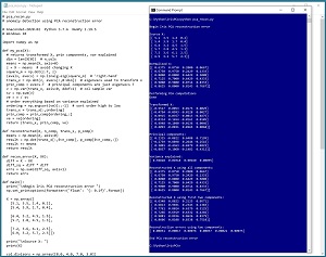 [Click on image for larger view.] Figure 1: Anomaly Detection Using PCA in Action
A good way to see where this article is headed is to take a look at the screen shot of a demo program shown in Figure 1. The demo sets up a dummy dataset of six items:
 [ 5.1  3.5  1.4  0.2]
 [ 5.4  3.9  1.7  0.4]
 [ 6.4  3.2  4.5  1.5]
 [ 5.7  2.8  4.5  1.3]
 [ 7.2  3.6  6.1  2.5]
 [ 6.9  3.2  5.7  2.3]
Each data item has four elements. The demo normalizes the data so that items with large elements don't dominate items with small elements:
 [ 0.6375  0.8750  0.2000  0.0667]
 [ 0.6750  0.9750  0.2429  0.1333]
 [ 0.8000  0.8000  0.6429  0.5000]
 [ 0.7125  0.7000  0.6429  0.4333]
 [ 0.9000  0.9000  0.8714  0.8333]
 [ 0.8625  0.8000  0.8143  0.7667]
The demo applies principal component analysis to the normalized data which results in four principal components. The first two of the four principal components are used to reconstruct the data:
 [ 0.6348  0.8822  0.2125  0.0571]
 [ 0.6813  0.9691  0.2343  0.1383]
 [ 0.7761  0.8024  0.6379  0.5125]
 [ 0.7266  0.6919  0.6332  0.4366]
 [ 0.9081  0.8936  0.8626  0.8379]
 [ 0.8606  0.8108  0.8338  0.7510]
The reconstructed data is compared to the original data by computing the sum of squared errors between elements. The six error values are (0.00031, 0.00017, 0.00076, 0.00037, 0.00021, 0.00075).
Error value [2] is the largest reconstruction error (0.00076) and therefore data item [2] (6.4, 3.2, 4.5, 1.5) is the most anomalous.
This article assumes you have an intermediate or better familiarity with a C-family programming language but doesn't assume you know anything about principal component analysis. The demo program is implemented using Python but you should be able to refactor to another language, such as C# or JavaScript, if you wish.
The complete source code for the demo program is presented in this article and is also available in the accompanying file download. All normal error checking has been removed to keep the main ideas as clear as possible.
To run the demo program, you must have Python installed on your machine. The demo program was developed on Windows 10 using the Anaconda 2020.02 64-bit distribution (which contains Python 3.7.6). The demo program has no significant dependencies so any relatively recent version of Python 3 will work fine.
Understanding PCA for Anomaly Detection
PCA is based on decomposition. Suppose that you want to decompose the integer value 64 into three components. There are many possible decompositions. One decomposition is (8, 4, 2) because 8 * 4 * 2 = 64. The first component, 8, accounts for most of the original value, the 4 accounts for less and the 2 accounts for the least amount. If you use all three components to reconstruct the source integer you will replicate the source exactly. But if you use just the first two components to reconstruct the source integer you will get a value that's close to the source: 8 * 4 = 32.
Principal component analysis is a very complex decomposition that works on data matrices instead of single integer values. In my opinion, PCA is best understood by examining a concrete example, such as the demo.
The six-item source dataset consists of six arbitrary items selected from the well-known 150-item Iris Dataset. Each item represents an iris flower and has four elements: sepal length and width (a sepal is a leaf-like structure), and petal length and width. Anomaly detection using PCA works only on strictly numeric data, which is the main limitation of the technique.
The source data is:
 [ 5.1  3.5  1.4  0.2]
 [ 5.4  3.9  1.7  0.4]
 [ 6.4  3.2  4.5  1.5]
 [ 5.7  2.8  4.5  1.3]
 [ 7.2  3.6  6.1  2.5]
 [ 6.9  3.2  5.7  2.3]
Because PCA is based on statistical variance, it's important to normalize the source data. The demo normalizes the data by the four columns by constants (8, 4, 7, 3) so that all values are between 0.0 and 1.0:
 [ 0.6375  0.8750  0.2000  0.0667]
 [ 0.6750  0.9750  0.2429  0.1333]
 [ 0.8000  0.8000  0.6429  0.5000]
 [ 0.7125  0.7000  0.6429  0.4333]
 [ 0.9000  0.9000  0.8714  0.8333]
 [ 0.8625  0.8000  0.8143  0.7667]
There are three results from PCA -- transformed data, principal components and variance explained. The transformed data is:
 [-0.5517  0.0053  0.0173  0.0029]
 [-0.4754 -0.0993 -0.0128  0.0027]
 [ 0.0915  0.0357 -0.0013 -0.0275]
 [ 0.0314  0.1654 -0.0161  0.0105]
 [ 0.4948 -0.1040 -0.0136  0.0046]
 [ 0.4093 -0.0031  0.0265  0.0068]
Notice the transformed data has the same shape as the original source data. The transformed data is an internal representation that can be used along with the principal components to reconstruct the original data.
The principal components are:
 [ 0.2325 -0.0822  0.6488  0.7199]
 [-0.2739 -0.8898  0.2646 -0.2516]
 [ 0.3001 -0.4363 -0.6979  0.4823]
 [-0.8837  0.1060 -0.1482  0.4312]
The principal components are stored in the columns and so the first component is (0.2325, -0.2739, 0.3001, -0.8837). The number of columns in the original data is sometimes called the dimension (dim) of the problem, so dim = 4 for the demo data. Each principal component has dim items and there are dim components. Put another way, the principal components matrix has shape dim x dim.
The principal components are stored so that the first component accounts for most of the statistical variance in the decomposition, the second component accounts for the second most variance and so on. For the demo, the percentages of the total variances accounted for are (0.94828, 0.04918, 0.00160, 0.00095). This means that the first principal component accounts for 94 percent of the total variance, the second accounts for 5 percent and the third and fourth components account for the remaining 1 percent of the total variance.
One way to think about the principal components is that they are a description, or alternative representation of, the source data. The demo program shows that if you use all the principal components to reconstruct the data, you will get the original source data back. This isn't useful for anomaly detection. If you use just some of the principal components to reconstruct the data, the reconstructed data will be close to the source data. The more principal components you use, the closer the reconstruction will be to the source. The demo uses the first two components to reconstruct the data:
 [ 0.6348  0.8822  0.2125  0.0571]
 [ 0.6813  0.9691  0.2343  0.1383]
 [ 0.7761  0.8024  0.6379  0.5125]
 [ 0.7266  0.6919  0.6332  0.4366]
 [ 0.9081  0.8936  0.8626  0.8379]
 [ 0.8606  0.8108  0.8338  0.7510]
The demo uses the sum of squared error between elements to compute a reconstruction error for each of the six data items. The six reconstruction error values are (0.00031, 0.00017, 0.00076, 0.00037, 0.00021, 0.00075).
For example, the first normalized source data item is (0.6375, 0.8750, 0.2000, 0.0667). Its reconstruction is (0.6348, 0.8822, 0.2125, 0.0571). The item error is: (0.6375 - 0.6348)^2 + (0.8750 - 0.8822)^2 + (0.2000 - 0.2125)^2 + (0.0667 - 0.0571)^2 = 0.00031.
The Demo Program
The complete demo program is presented in Listing 1. The program begins by setting up the source data:
import numpy as np

def main():
  print("Begin Iris PCA reconstruction error ")
  X = np.array([
    [5.1, 3.5, 1.4, 0.2],
    [5.4, 3.9, 1.7, 0.4],
    [6.4, 3.2, 4.5, 1.5],
    [5.7, 2.8, 4.5, 1.3],
    [7.2, 3.6, 6.1, 2.5],
    [6.9, 3.2, 5.7, 2.3]])
. . .
The demo data is hard-coded. In a non-demo scenario, you would likely read the source data into memory from file using np.loadtxt() or a similar function.
Listing 1: Complete Anomaly Detection Demo Program
# pca_recon.py
# anomaly detection using PCA reconstruction error

# Anaconda3-2020.02  Python 3.7.6  NumPy 1.19.5
# Windows 10

import numpy as np

def my_pca(X):
  # returns transformed X, prin components, var explained
  dim = len(X[0])  # n_cols
  means = np.mean(X, axis=0)
  z = X - means  # avoid changing X
  square_m = np.dot(z.T, z)
  (evals, evecs) = np.linalg.eig(square_m)
  trans_x = np.dot(z, evecs[:,0:dim])
  prin_comp = evecs.T
  v = np.var(trans_x, axis=0, ddof=1)  # sample var
  sv = np.sum(v)
  ve = v / sv
  # order everything based on variance explained
  ordering = np.argsort(ve)[::-1]  # sort high to low
  trans_x = trans_x[:,ordering]
  prin_comp = prin_comp[ordering,:]
  ve = ve[ordering]
  return (trans_x, prin_comp, ve)

def reconstructed(X, n_comp, trans_x, p_comp):
  means = np.mean(X, axis=0)
  result = np.dot(trans_x[:,0:n_comp], p_comp[0:n_comp,:])
  result += means
  return result

def recon_error(X, XX):
  diff = X - XX
  diff_sq = diff * diff
  errs = np.sum(diff_sq, axis=1)
  return errs

def main():
  print("\nBegin Iris PCA reconstruction error ")
  np.set_printoptions(formatter={'float': '{: 0.1f}'.format})

  X = np.array([
    [5.1, 3.5, 1.4, 0.2],
    [5.4, 3.9, 1.7, 0.4],

    [6.4, 3.2, 4.5, 1.5],
    [5.7, 2.8, 4.5, 1.3],

    [7.2, 3.6, 6.1, 2.5],
    [6.9, 3.2, 5.7, 2.3]])

  print("\nSource X: ")
  print(X)

  col_divisors = np.array([8.0, 4.0, 7.0, 3.0])
  X = X / col_divisors
  print("\nNormalized X: ")
  np.set_printoptions(formatter={'float': '{: 0.4f}'.format})
  print(X)

  print("\nPerforming PCA computations ")
  (trans_x, p_comp, ve) = my_pca(X)
  print("Done ")

  print("\nTransformed X: ")
  np.set_printoptions(formatter={'float': '{: 0.4f}'.format})
  print(trans_x)

  print("\nPrincipal components: ")
  np.set_printoptions(formatter={'float': '{: 0.4f}'.format})
  print(p_comp)

  print("\nVariance explained: ")
  np.set_printoptions(formatter={'float': '{: 0.5f}'.format})
  print(ve)

  XX = reconstructed(X, 4, trans_x, p_comp)
  print("\nReconstructed X using all components: ")
  np.set_printoptions(formatter={'float': '{: 0.4f}'.format})
  print(XX)

  XX = reconstructed(X, 2, trans_x, p_comp)
  print("\nReconstructed X using first two components: ")
  np.set_printoptions(formatter={'float': '{: 0.4f}'.format})
  print(XX)

  re = recon_error(X, XX)
  print("\nReconstruction errors using two components: ")
  np.set_printoptions(formatter={'float': '{: 0.5f}'.format})
  print(re)

  print("\nEnd PCA reconstruction error ")
if __name__ == "__main__":
  main()
Next, the demo normalizes the source data by dividing each column by a constant that will yield values between 0.0 and 1.0:
  col_divisors = np.array([8.0, 4.0, 7.0, 3.0])
  X = X / col_divisors
The demo modifies the source data. In some scenarios you might want to create a new matrix of normalized values in order to leave the original source data unchanged. Alternative normalization techniques include min-max normalization and z-score normalization. If you don't normalize the source data, the reconstruction error will be dominated by the column that has the largest magnitude values.
The principal component analysis is performed by a call to a program-defined my_pca() function:
  print("Performing PCA computations ")
  (trans_x, p_comp, ve) = my_pca(X)
  print("Done ")
The return result is a tuple with three values. The trans_x is the internal transformed data that is needed to reconstruct the data. The p_comp is the principal components matrix where components are stored in the columns. The ve is a vector of percentages of variance explained. The my_pca() function is implemented so that the principal components are stored in order from most variance explained to least variance explained.
The demo reconstructs the data using a program-defined reconstructed() function:
  XX = reconstructed(X, 4, trans_x, p_comp)
  . . .
  XX = reconstructed(X, 2, trans_x, p_comp)
The first call to reconstructed() uses all 4 principal components and so the source normalized data is reconstructed exactly. The second call uses just the first 2 principal components so the reconstructed data is close to but, not exactly the same as, the source data.
The demo concludes by computing a vector of the reconstruction errors for each data item using a program-defined recon_error() function:
. . .
  re = recon_error(X, XX)
  print("Reconstruction errors using two components: ")
  np.set_printoptions(formatter={'float': '{: 0.5f}'.format})
  print(re)

  print("End PCA reconstruction error ")
if __name__ == "__main__":
  main()
In a non-demo scenario, you'd likely sort the error values from largest to smallest to get the top-n anomalous data items.
Behind the Scenes
The key statements in the program-defined my_pca() function are:
def my_pca(X):
  dim = len(X[0])  # number cols
  means = np.mean(X, axis=0)
  z = X - means  # avoid changing X
  square_m = np.dot(z.T, z)
  (evals, evecs) = np.linalg.eig(square_m)  # 'right-hand'
  trans_x = np.dot(z, evecs[:,0:dim])
  prin_comp = evecs.T
  # compute variance explained, sort everything
  . . .
  return (trans_x, prin_comp, ve)
The heart of the PCA function is a call to the NumPy linalg.eig() function ("linear algebra, eigen"). The function returns an eigenvalues array and an eigenvectors matrix. The eig() function is very complex and implementing it from scratch is possible but usually not practical. The principal components are the (transposed) eigenvectors, and the transformed internal representation matrix is the product of a square matrix derived from the source data and the eigenvectors. The Wikipedia article on Eigenvalues and Eigenvectors has a complicated but thorough explanation.
The implementation of the program-defined reconstructed() function is:
def reconstructed(X, n_comp, trans_x, p_comp):
  means = np.mean(X, axis=0)
  result = np.dot(trans_x[:,0:n_comp], p_comp[0:n_comp,:])
  result += means
  return result
The reconstructed data matrix is the matrix product of the transformed data and the principal components. The means of the columns are added because means were subtracted by the PCA function.
Using the Scikit Library
The scikit-learn code library has a high-level wrapper function for PCA that can be used instead of the program-defined my_pca() function. Code to use the scikit function could be:
import sklearn.decomposition
pca = sklearn.decomposition.PCA().fit(X)
trans_x = pca.transform(X)
p_comp = pca.components_
ve = pca.explained_variance_ratio_
The PCA class transform() method returns the internal transformed data (for reconstruction), and stores the principal components matrix and percentage of variance explained vector as class members.
Using the scikit library is somewhat simpler than implementing a program-defined my_pca() function. But using scikit introduces an external library dependency. External dependencies have a way of biting you months later when your code suddenly stops working because of breaking change to an implementation or API signature.
Wrapping Up
Anomaly detection using principal component analysis reconstruction is one of the oldest unsupervised anomaly detection techniques, dating from the early 1900s. The main advantage of using PCA is simplicity, assuming you have a function that computes eigenvalues and eigenvectors. The two main disadvantages of using PCA are 1.) the technique works only with strictly numeric data, and 2.) because PCA uses matrices in memory, the technique does not scale to very large datasets.
Among my colleagues, anomaly detection using PCA reconstruction error has been largely replaced by deep neural autoencoder reconstruction error. However, PCA is often useful as a baseline because the technique only requires a single hyperparameter, the number of principal components to use for the reconstruction.