The Data Science Lab
Matrix Inverse Using Cayley-Hamilton with C#
Dr. James McCaffrey presents a complete end-to-end demonstration of computing a matrix inverse using the Cayley-Hamilton technique. Compared to other matrix inverse algorithms, Cayley-Hamilton is by far the simplest and as a nice side effect gives you the matrix determinant. However, Cayley-Hamilton is not suitable for large matrices.
Dozens of machine learning algorithms require computing the inverse of a matrix. Computing a matrix inverse is conceptually easy, but implementation is one of the most challenging tasks in numerical programming.
The Wikipedia article on matrix inverse lists 14 different algorithms, and each algorithm has multiple variations, and each variation has dozens of implementation alternatives. Four examples include:
- LUP decomposition algorithm (Crout version and others)
- QR decomposition algorithm (Householder version and others)
- SVD decomposition algorithm (Jacobi version and others)
- Cholesky decomposition (Banachiewicz version and others)
The fact that there are so many different techniques is a direct indication of how tricky it is to compute a matrix inverse.
This article presents a complete end-to-end demonstration of computing a matrix inverse using a technique called Cayley-Hamilton. Compared to other algorithms, Cayley-Hamilton is very simple and easiest to customize. The main disadvantage of Cayley-Hamilton is that it's not suitable for matrices larger than about 200-by-200, and the algorithm can easily fail even for small matrices.
In ordinary arithmetic, 0.125 is the inverse of 8 because 0.125 * 8 = 1. In matrix algebra, the inverse of some matrix A is a matrix Ainv if A * Ainv = Ainv * A = I, where * indicates matrix multiplication, and I is the identity matrix (1.0 values on the upper-left to lower-right diagonal, 0.0 values elsewhere). Matrix inverse applies only to square matrices (equal number of rows and columns). Not all square matrices have an inverse.
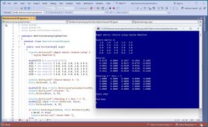 [Click on image for larger view.] Figure 1: Computing a Matrix Inverse Using Cayley-Hamilton
A good way to see where this article is headed is to take a look at the screenshot of a demo program in Figure 1. The demo begins by setting up a 5-by-5 matrix:
Begin matrix inverse using Cayley-Hamilton

Source matrix A:
   1.0   2.0   3.0   1.0   5.0
   0.0   5.0   4.0   1.0   4.0
   6.0   1.0   0.0   2.0   2.0
   1.0   4.0   5.0   3.0   2.0
   0.0   2.0   4.0   0.0   1.0
Next, the demo computes and displays the inverse of the source matrix:
Inverse:
  -0.0738   0.0000   0.1967  -0.1066   0.1885
  -0.2984   0.4000   0.0623  -0.0754  -0.0820
   0.0836  -0.2000  -0.0230   0.0541   0.3197
   0.1082  -0.2000  -0.0885   0.4230  -0.4098
   0.2623   0.0000  -0.0328  -0.0656  -0.1148
The demo program concludes by verifying that the computed inverse is correct:
Checking A * Ainv = I
   1.0000   0.0000   0.0000   0.0000   0.0000
   0.0000   1.0000   0.0000   0.0000   0.0000
   0.0000   0.0000   1.0000   0.0000   0.0000
   0.0000   0.0000   0.0000   1.0000   0.0000
   0.0000   0.0000   0.0000   0.0000   1.0000

Check PASS

End demo
Behind the scenes, the demo program calls a function MatAreEqual() that compares A * Ainv with the identity matrix to check that all the values in the two matrices are the same to within a 1.0e-8 tolerance.
This article assumes you have intermediate or better programming skill but doesn't assume you know anything about the Cayley-Hamilton technique for computing the inverse of a matrix. The demo is implemented using C# but you should be able to refactor the demo code to another C-family language if you wish. Most normal error checking has been removed to keep the main ideas as clear as possible.
The source code for the demo program is a bit too long to be presented in its entirety in this article. The complete code is available in the accompanying file download, and is also available online.
Understanding the Cayley-Hamilton Matrix Inverse Technique
Suppose you have a 5-by-5 square matrix A that can be inverted. The first step is to compute the so-called coefficients of the characteristic polynomial of A. There are several ways to do this, but for now, just assume you can get the coefficients.
For a 5-by-5 matrix there will be 6 coefficients stored in a vector c. The first cell of c, c[0], will always hold a 1.0 value. For the demo matrix A, it turns out that the coefficients are:
 1  -10  -21  37  373  -610
 0    1    2   3   4     5
The inverse of matrix A is (A^4 - 10*A^3 - 21*A^2 + 37*A + 373*I) / 610
The A^4 means A * A * A * A. Cell coefficient c[0] is always 1 and can be ignored (or you can imagine it is associated with the A^4 term). Cell c[1] goes with A^3, cell c[2] goes with A^2, cell c[3] goes with A. The next to last cell, c[4] goes with I, the identity matrix. The last cell, c[5] is the negative of a final division scaling factor.
If you examine this example for a bit, you should see the pattern. Putting this together for a matrix A with size n-by-n gives a stunningly short function to compute an inverse. The math for Cayley-Hamilton is very complicated, but from a software engineering perspective, you only need to know the final pattern.
This example points out one of the key weaknesses of Cayley-Hamilton. For the 5-by-5 demo matrix, you need to compute powers of A up to A^4. So, for a 100-by-100 matrix, you'd need to compute powers of A up to 99. This is time-consuming and is subject to round off errors and arithmetic overflow and underflow. In practice, you can use Cayley-Hamilton for matrices up to about size 200, but the exact maximum feasible size varies a lot depending on the values in the source matrix.
The simplicity of Cayley-Hamilton matrix inverse depends on being able to compute the coefficients of the characteristic polynomial. This is another very deep math topic but fortunately one that can be implemented relatively easily. There are several algorithms to compute the coefficients but the easiest, and the one used by the demo program, is called the Faddeev-LeVerrier algorithm.
The implementation is:
public static double[] MatPoly(double[][] A) {
  int n = A.Length;
  double[] c = new double[n + 1]; c[0] = 1.0;
  double[][] Ak = MatCopyOf(A);
  for (int k = 1; k <= n; ++k)  {
    double ck = -1 * MatTrace(Ak) / k;
    c[k] = ck;
    for (int i = 0; i < n; ++i)
      Ak[i][i] += ck;
    Ak = MatMult(A, Ak);
  }
  return c;
}
Notice that for an n-by-n matrix, the result coefficients are in a vector with n+1 cells. The MatTrace() function computes the sum of matrix values on the upper-left to lower-right diagonal. I can't think of any scenarios where you'd want to modify the MatPoly() function, so you can think of it as a black box.
The Demo Program
I used Visual Studio 2022 (Community Free Edition) for the demo program. I created a new C# console application and checked the "Place solution and project in the same directory" option. I specified .NET version 8.0. I named the project MatrixInverseCayleyHamilton. I checked the "Do not use top-level statements" option to avoid the weird program entry point shortcut syntax.
The demo has no significant .NET dependencies and any relatively recent version of Visual Studio with .NET (Core) or the older .NET Framework will work fine. You can also use the Visual Studio Code program if you like.
After the template code loaded into the editor, I right-clicked on file Program.cs in the Solution Explorer window and renamed the file to the more descriptive MatrixInverseCHProgram.cs. I allowed Visual Studio to automatically rename class Program.
The overall program structure is presented in
Listing 1. All the control logic is in the Main() method in the Program class. All of the matrix inverse functionality is contained in static functions/methods in a Utils class.
Listing 1: Overall Program Structure
using System;
using System.IO;
using System.Collections.Generic;

namespace MatrixInverseCayleyHamilton
{
  internal class MatrixInverseCHProgram
  {
    static void Main(string[] args)
    {
      Console.WriteLine("Begin matrix inverse using" +
        " Cayley-Hamilton");

      // 1. set up and display source matrix
      // 2. compute and display the inverse
      // 3. verify the inverse is correct

      Console.WriteLine("End demo ");
      Console.ReadLine();
    }
  }

  // ========================================================

  public class Utils
  {
    // ------------------------------------------------------

    public static double[][]
      MatInverseCayleyHamilton(double[][] A) { . . }

    public static double[] MatPoly(double[][] A) { . . }

    public static double[][] MatMake(int nRows,
      int nCols) { . . }

    public static void MatShow(double[][] A, int dec,
      int wid) { . . }

    public static double[][] MatLoad(string fn, int[] usecols,
      char sep, string comment) { . . }

    public static double[][] MatMult(double[][] A,
      double[][] B) { . . }

    public static double[][] MatAdd(double[][] A,
      double[][] B) { . . }

    public static double MatTrace(double[][] A) { . . }

    public static double[][] MatCopyOf(double[][] A) { . . }

    public static double[][] MatScalarMult(double u,
      double[][] A) { . . }

    public static double[][] MatIdentity(int n) { . . }

    public static bool MatAreEqual(double[][] A,
      double[][] B, double eps) { . . }
  }

  // ========================================================

} // ns
The demo program begins by setting up a source matrix using these statements:
double[][] A = new double[5][];
A[0] = new double[] { 1.0, 2.0, 3.0, 1.0, 5.0 };
A[1] = new double[] { 0.0, 5.0, 4.0, 1.0, 4.0 };
A[2] = new double[] { 6.0, 1.0, 0.0, 2.0, 2.0 };
A[3] = new double[] { 1.0, 4.0, 5.0, 3.0, 2.0 };
A[4] = new double[] { 0.0, 2.0, 4.0, 0.0, 1.0 };

Console.WriteLine("Source matrix A: ");
Utils.MatShow(A, 1, 6);  // 1 decimal, 6 wide
The demo defines a matrix as an array of arrays of type double. It's possible to use a program-defined matrix class, but in my opinion this approach creates unnecessary complexity. The most recent versions of .NET allow you to use a shortcut syntax to initialize an array, for example, A[0] = [1.0, -2.0, 3.0, 1.0, 5.0] but using this syntax creates a version dependency.
You access each cell of an array-of-arrays style using syntax like A[0][2] = 3.45 where the first index is the row and the second index is the column. Unlike most programming languages, C# also has a 2D array type that is accessed like A[0,2] = 3.45 but I do not recommend using this data type mostly because almost all published matrix algorithms assume an array-of-arrays style matrix.
In a non-demo scenario, you might want to load data into a matrix from a text file. The demo code has a MatLoad() function that isn't used but could be called like:
string fn = "dummy_data.txt";
double[][] A = Utils.MatLoad(fn,
  new int[] { 0, 1, 2, 3, 4 }, ',', "#");
This syntax means load the data in file dummy_data.txt, using columns [0] to [4], where the data is delimited by the comma character, and comments to be ignored are lines that begin with the # character.
Computing the Matrix Inverse
The demo program computes and displays the inverse of the source matrix using these statements:
double[][] Ainv = Utils.MatInverseCayleyHamilton(A);
Console.WriteLine("Inverse: ");
Utils.MatShow(Ainv, 4, 9);
The code for the Utils.MatInverseCayleyHamilton() function is shown in Listing 2. The code presented in this article is explicitly intended for you to modify to meet your needs. For example, you might want to verify that the source matrix A has the same number of rows and columns. Or you might want to refactor the code to put the MatPoly() functionality directly into the MatInverseCayleyHamilton() function.
Listing 2: The MatInverseCayleyHamilton Function
public static double[][] MatInverseCayleyHamilton(double[][] A)
{
  int n = A.Length; // A must be square
  double[] coeffs = MatPoly(A);
  double[][] Apower = MatCopyOf(A);
  double[][] result = MatScalarMult(coeffs[n - 1], MatIdentity(n));
  int k = n - 2;
  while (k >= 0)  {
    result = MatAdd(result, MatScalarMult(coeffs[k], Apower));
    Apower = MatMult(Apower, A);
    --k;
  }
  result = MatScalarMult(-1 / coeffs[n], result);
  return result;
}
An interesting side effect of the Cayley-Hamilton technique is that when you compute the coefficients of the characteristic polynomial, you also compute the determinant of the source matrix. The determinant magnitude is stored in the last cell of the coefficients vector, coeffs[n]. If the size of the matrix n is even, the determinant is just coeffs[n]. If n is odd, then the determinant is -1 * coeffs[n]. So for the demo program with n = 5, which is odd, the determinant is -1 * -610 = 610.
You could modify the MatInverseCayleyHamilton() function to return the determinant as an out parameter:
public static double[][] MatInverseCayleyHamilton(double[][] A,
  out double det)
{
. . .
  if (n % 2 == 0)
    det = coeffs[n];
  else
    det = -1 * coeffs[n];
  return result;
}
And then you could call like:
double det;
MatInverseCayleyHamilton(A, out det);
Console.WriteLine("Determinant is " + det);
Most of the technical references on Cayley-Hamilton determinant computation expresses the value as (-1)^n * coeffs[n] which gives the same result as the even/odd approach.
Checking the Matrix Inverse
The demo concludes by checking that the computed matrix inverse is correct:
Console.WriteLine("Checking A * Ainv = I ");
double[][] check = Utils.MatMult(A, Ainv);
Utils.MatShow(check, 4, 9);

if (Utils.MatAreEqual(check, Utils.MatIdentity(5), 1.0e-8) == true)
  Console.WriteLine("Check PASS ");
else
  Console.WriteLine("Check FAIL ");
Recall that for a source matrix A, the definition of a matrix inverse Ainv is one where A * Ainv = Ainv * A = I. The demo program checks just A * Ainv. In a non-demo scenario, it'd be more thorough to also check Ainv * A.
The Cayley-Hamilton technique can fail in many ways, which is why it's not used very often. The first point of possible failure is computing the coefficients of the characteristic polynomial. If the source matrix is large, and all the cells are positive (such as a machine learning Kernel matrix), the MatTrace() result can easily overflow.
In a non-demo scenario, you should examine the coefficients to make sure none of them has exploded to a huge value, or shrunk to nearly zero. Cayley-Hamilton usually works best when the source matrix has small magnitude values that are both positive and negative.
Wrapping Up
Compared to other matrix inverse algorithms, the Cayley-Hamilton technique is easy to modify and is highly interpretable if you insert diagnostic print statements. The main disadvantage of Cayley-Hamilton is that is slow. Here are some timing results for inverting dim-by-dim matrices filled with random values between -1.0 and +1.0, using a check tolerance of 1.0e-8, run on a standard desktop machine:
 dim     time
-------------------
  10     0.0 seconds
  50     0.1 seconds
 100     1.2 seconds
 200    20.8 seconds
 300   115.2 seconds ( ~2 minutes)
 400   434.2 seconds ( ~7 minutes)
 500  1223.0 seconds (~20 minutes)
The time required to invert a matrix using Cayley-Hamilton is dominated by calls to the MatMult() function which requires approximately (dim * dim * dim) operations. Therefore, time increases exponentially and at some point, around size 500-by-500, Cayley-Hamilton becomes impractical.