Neural Network Lab

Neural Network Weight Decay and Restriction

Weight decay and weight restriction are two closely related, optional techniques that can be used when training a neural network. This article explains exactly what weight decay and weight restriction are, and how to use them with an existing neural network application or implement them in a custom application.

• By James McCaffrey
• 07/28/2014

The idea of weight decay is deceptively simple. In each training loop iteration, after the neural network's weights and bias values are updated, the weights and biases are decreased by a small amount. This tends to keep the magnitudes of the weight and bias values small, which in turn prevents over-fitting. The idea of weight restriction is similar. After the update and decay operations, the resulting weights and bias values are checked, and if too large or too small, the values are brought back into range. This process keeps weight and bias values small.

Also, the ideas are simple, but weight decay and restriction are often coded incorrectly in neural network implementations. And, as you'll see shortly, the weight decay parameter can have more than one interpretation, which can lead to some confusion when working with commercial or open source neural network tools.

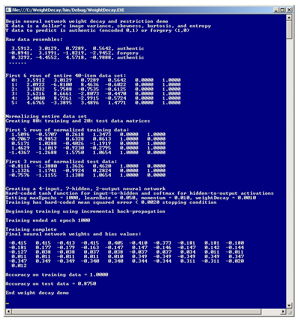
To get a feel for where this article is headed, take a look at the demo program in Figure 1. The demo trains a neural network that classifies a banknote (think dollar bill) as authentic or a forgery based on four properties of a photographic image of the banknote. The data set consists of 40 items. The independent x values represent a banknote's image variance, skewness, kurtosis, and entropy. You can just think of these as numeric characteristics without worrying about their exact meaning. The demo encodes dependent y value authentic as (0, 1) and forgery as (1, 0).

The demo normalizes the data set, which is extremely important when using weight decay and restriction. The data is split into an 80 percent (32 items) training set and a 20 percent (8 items) test set. The demo creates a 4-7-2 neural network. The neural network uses weight decay and restriction during training. The neural network correctly classifies all 32 training banknotes, and then using the weights and bias values found during training, correctly classifies 87.50 percent (7 out of 8) of the test banknotes.

This article assumes you have at least intermediate-level programming skills and a solid grasp of basic neural network training concepts, but doesn't assume you know anything about weight decay and restriction. The demo is coded using C#, but you should be able to refactor the code to most other languages without too much difficulty. The demo code is too long to present here in its entirety, but the entire source code is available in the download accompanying this article.

Overall Program Structure
The structure of the demo program, with some minor edits, is presented in Listing 1. The structure is fairly large because the demo is a fully function neural network. However, weight decay and restriction appear only in a few of the neural network's methods. To create the demo I launched Visual Studio and created a new C# console application named WeightDecay. In the Solution Explorer window I renamed the file Program.cs to WeightDecayProgram.cs and Visual Studio renamed the class Program for me. At the top of the source code I removed all unnecessary using statements.

using System;
namespace WeightDecay
{
  class Program
  {
    static void Main(string[] args)
    {
      Console.WriteLine("Begin weight decay demo");

      // Set up all data here
      // Normalize data
      // Split data into train and test

      int numInput = 4;
      int numHidden = 7;
      int numOutput = 2;
      NeuralNetwork nn =
        new NeuralNetwork(numInput, numHidden, numOutput);

      int maxEpochs = 1000;
      double learnRate = 0.05;
      double momentum = 0.01;
      double weightDecay = 0.001;

      nn.Train(trainData, maxEpochs, learnRate,
        momentum, weightDecay);
      Console.WriteLine("Training complete");

      // Fetch resulting weights and bias values
      // Compute accuracy of training and test sets

      Console.WriteLine("End weight decay demo");
      Console.ReadLine();
    }

    static void Normalize(double[][] dataMatrix, int[] cols) { . . }
    static void MakeTrainTest(double[][] allData, int seed,
      out double[][] trainData, out double[][] testData) { . . }
    static void ShowVector(double[] vector, int valsPerRow,
      int decimals, bool newLine) { . . }
    static void ShowMatrix(double[][] matrix, int numRows,
      int decimals, bool lineNums, bool newLine) { . . }
  }

  public class NeuralNetwork
  {
    private static Random rnd;

    private int numInput;
    private int numHidden;
    private int numOutput;

    private double[] inputs;

    private double[][] ihWeights; // input-hidden
    private double[] hBiases;
    private double[] hOutputs;

    private double[][] hoWeights; // hidden-output
    private double[] oBiases;

    private double[] outputs;

    private double[] oGrads; // output gradients
    private double[] hGrads; // hidden gradients

    private double[][] ihPrevWeightsDelta; 
    private double[] hPrevBiasesDelta;
    private double[][] hoPrevWeightsDelta;
    private double[] oPrevBiasesDelta;

    public NeuralNetwork(int numInput, int numHidden,
      int numOutput) { . . }
    private static double[][] MakeMatrix(int rows,
      int cols) { . . }
    public void SetWeights(double[] weights) { . . }
    private void InitializeWeights() { . . }
    public double[] GetWeights() { . . }
    private double[] ComputeOutputs(double[] xValues) { . . }
    private static double HyperTanFunction(double x) { . . }
    private static double[] Softmax(double[] oSums) { . . }
    private void UpdateWeights(double[] tValues,
      double learnRate, double momentum, double weightDecay) { . . }
    public void Train(double[][] trainData, int maxEprochs,
      double learnRate, double momentum, double weightDecay) { . . }
    private static void Shuffle(int[] sequence) { . . }
    private double MeanSquaredError(double[][] trainData) { . . }
    public double Accuracy(double[][] testData) { . . }
    private static int MaxIndex(double[] vector) { . . }
  }
} // ns

After some preliminary WriteLine statements, the Main method begins by setting up the banknote data:

static void Main(string[] args)
{
  double[][] allData = new double[40][];
  allData[0] = new double[] { 3.5912, 3.0129, 0.7289, 0.5642, 0, 1 };
  allData[1] = new double[] { 2.0922, -6.8100, 8.4636, -0.6022, 0, 1 };
  // And so on
  allData[38] = new double[] { -1.8215, 2.7521, -0.7226, -2.3530, 1, 0 };
  allData[39] = new double[] { -1.6677, -7.1535, 7.8929, 0.9677, 1, 0 };
...

The data used here is a randomly selected 40-item subset of the 1372-item banknote authentication data set, which is available from the UCI machine learning data repository. The original set encodes authentic as 0 and forgery as 1. The demo encodes authentic as (0, 1) and forgery as (1, 0).

Next, the demo normalizes the data:

Console.WriteLine("First 6 rows of entire 40-item data set:");
ShowMatrix(allData, 6, 4, true, true);

Console.WriteLine("Normalizing entire data set");
Normalize(allData, new int[] { 0, 1, 2, 3 });

The Normalize method accepts a matrix of data and an array of column indices. The method performs a Gaussian normalization on the specified columns by subtracting the column mean from each value and then dividing by the column standard deviation. The resulting matrix is then scaled so that all the values have roughly the same magnitude. If you don't normalize your x data, columns with very large values can overwhelm columns with small values. Notice that method Normalize returns void and operates directly on its input matrix parameter; you may want to return the normalized result instead.

Next, the demo randomly splits the 40-item normalized data into a 32-item training matrix and an eight-item test matrix:

Console.WriteLine("Creating 80% training and 20% test");
double[][] trainData = null;
double[][] testData = null;
MakeTrainTest(allData, 41, out trainData, out testData);
Console.WriteLine("First 5 rows of normalized training data:");
ShowMatrix(trainData, 5, 4, false, true);
Console.WriteLine("First 3 rows of normalized test data:");
ShowMatrix(testData, 3, 4, false, true);

The mysterious looking 41 parameter value is the seed for the randomization process. That value was used only because it gave a nice-looking demo.

After dealing with the data, the demo instantiates as 4-7-2 neural network as shown in Listing 1. The 4 and 2 values are defined by the structure of the data -- four x values and two y values. The problem being addressed is a binary classification problem -- that is, there are two possible classes: authentic and forgery. For binary classification problems, it's most common to just encode the two possible y values as 0 and 1, and use the logistic sigmoid activation function for the output layer node. However, there's some research that suggests when using weight decay and restriction on a binary classification problem, it's preferable to use two output nodes and softmax activation. I'm not completely convinced by the research in this area, and in my opinion, the best approach to use is still an open question.

The demo prepares and executes training like so:

int maxEpochs = 1000;
double learnRate = 0.05;
double momentum = 0.01;
double weightDecay = 0.001;
// Echo parameter values
Console.WriteLine("Beginning training using back-propagation");
nn.Train(trainData, maxEpochs, learnRate, momentum, weightDecay);
Console.WriteLine("Training complete");

The demo uses the back-propagation algorithm, but weight decay and restriction can be used with any training algorithm. The weightDecay parameter is set to value 0.001. As with the other training parameters, finding a good value of the weightDecay parameter is essentially a matter of trial and error. Notice there's no parameter associated with weight restriction; the restriction parameter is hardcoded inside the UpdateWeights method.

After training, the demo retrieves the resulting weights and bias values:

double[] weights = nn.GetWeights();
Console.WriteLine("Final neural network weights and bias values:");
ShowVector(weights, 10, 3, true);

The demo concludes by computing the accuracy of the resulting neural network on the training and test data:

  double trainAcc = nn.Accuracy(trainData);
  Console.WriteLine("Accuracy on training data = " +
    trainAcc.ToString("F4"));

  double testAcc = nn.Accuracy(testData);
  Console.WriteLine("Accuracy on test data = " +
    testAcc.ToString("F4"));

  Console.WriteLine("End weight decay demo");
  Console.ReadLine();
} // Main

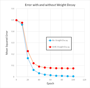
To see how weight decay and restriction can affect neural network training, take a look at the graph of the demo program error in Figure 2. Including weight decay tends to increase the time required to train, but the final neural network model tends to generalize better on new data.

The effect in Figure 2 is relatively magnified because the demo problem is so small. On larger, more realistic classification problems, using weight decay often has less of an impact on performance.

Understanding Weight Decay
Weight decay is probably best explained using a concrete example. Suppose some weight has an initial value of 3.000. The idea of weight decay is to iteratively reduce the magnitude of the value so that the value doesn't become extremely large or extremely small during training. Suppose the weight decay parameter has value 0.10 (in real life, weight decay parameters are typically much smaller). The weight value will be decreased by 0.10 (10 percent) in each iteration. For example:

3.000 -> 3.000 - (0.10)(3.000) = 3.000 - 0.300 = 2.700
2.700 -> 2.700 - (0.10)(2.700) = 2.700 - 0.270 = 2.430
2.430 -> 2.430 - (0.10)(2.430) = 2.430 - 0.243 = 2.187
and so on

Now, observe that subtracting 0.10 of the current weight value in each iteration is equivalent to multiplying by 0.90 in each iteration:

3.000 -> 3.000 * 0.90 = 2.700
2.700 -> 2.700 * 0.90 = 2.430
2.430 -> 2.430 * 0.90 = 2.187
and so on

The point here is that, when using commercial or open source neural network systems, you have to be careful to distinguish between weight decay parameters that represent an amount to subtract (0.10 in the example above), and those that represent a multiplication factor (0.90 in the example).

At first thought, weight decay has the feel of a hack. But weight decay is based on some solid mathematics. Using some fancy math footwork, it can be shown that if lambda represents a theoretical weight decay, then the amount a weight wt should be adjusted is given by:

wt' = wt * (eta * lambda)

where the meaning of eta can vary from reference to reference. The point here is that the weight decay parameter value can have different meanings in different contexts.

Implementing Weight Decay and Restriction
Weight decay and restriction are implemented in method UpdateWeights. The method's definition begins by computing the gradients of the output nodes. Gradients are measures of how far off, and in what direction, computed outputs are from the target desired output values in the training data:

private void UpdateWeights(double[] tValues, double learnRate,
  double momentum, double weightDecay)
{
  for (int i = 0; i < oGrads.Length; ++i) {
    double derivative = (1 - outputs[i]) * outputs[i];
    oGrads[i] = derivative * (tValues[i] - outputs[i]);
  }
... 

Next, the hidden layer node gradients are computed:

for (int i = 0; i < hGrads.Length; ++i) {
  double derivative = (1 - hOutputs[i]) * (1 + hOutputs[i]);
  double sum = 0.0;
  for (int j = 0; j < numOutput; ++j) {
    double x = oGrads[j] * hoWeights[i][j];
    sum += x;
  }
  hGrads[i] = derivative * sum;
}

The computation of the hidden node gradients assumes the hyperbolic tangent function is used for activation. Next, the input-to-hidden weights are computed, using weight decay and weight restriction, as shown in Listing 2.

for (int i = 0; i < numInput; ++i) {
  for (int j = 0; j < numHidden; ++j) {
    double delta = learnRate * hGrads[j] * inputs[i];
    ihWeights[i][j] += delta;
    ihWeights[i][j] += momentum * ihPrevWeightsDelta[i][j];
          
    ihWeights[i][j] -= (weightDecay * ihWeights[i][j]);

    if (ihWeights[i][j] < -10.0)
      ihWeights[i][j] = -10.0;
    else if (ihWeights[i][j] > 10.0)
      ihWeights[i][j] = 10.0;

    ihPrevWeightsDelta[i][j] = delta;
  }
}

Notice the weight decay isn't conditioned on whether the current weight value is negative or positive. A common mistake is to implement weight decay along the lines of:

if (ihWeights[i][j] > 0.0)
  ihWeights[i][j] -= (weightDecay * ihWeights[i][j]);
else
  ihWeights[i][j] += (weightDecay * ihWeights[i][j]);

This approach is incorrect. The weight decay parameter value is always positive. So, if the current weight value is positive, the product of the weight and the decay will be positive and subtracting that product will correctly reduce the magnitude of the weight. But if the current weight value is negative, the product of the weight and the decay will be negative. Adding a negative value to the current negative weight will make the weight even more negative, which is not the desired behavior.

The weight restriction thresholds are hardcoded as -10.0 and +10.0. One of the reasons why restriction thresholds can be hardcoded in the demo is because the data has been normalized. Because all the x values have roughly the same magnitude, in most cases the weights and bias values will also have roughly the same magnitude. The (-10.0, +10.0) values are to a large extent arbitrary, and there are some classification problems where weight restriction doesn't work well.

Next, method UpdateWeights deals with the hidden node biases:

for (int i = 0; i < numHidden; ++i) {
  double delta = learnRate * hGrads[i];
  hBiases[i] += delta;
  hBiases[i] += momentum * hPrevBiasesDelta[i];

  // hBiases[i] -= (weightDecay * hBiases[i]); // No !?

  if (hBiases[i] < -10.0)
    hBiases[i] = -10.0;
  else if (hBiases[i] > 10.0)
    hBiases[i] = 10.0;

  hPrevBiasesDelta[i] = delta;
}

Interestingly, even though biases are essentially weights with dummy 1.0 input values, it's standard practice to not apply decay to the hidden node and output node biases. There's very little research on this topic. In my experience, I haven't found much practical difference between applying and not applying weight decay to neural network biases.

Method UpdateWeights follows the same pattern to apply weight decay to the hidden-to-output weights, and skips applying decay to the output node biases. Check the code download for details.

Mixed Opinions
Among my colleagues who work with neural networks, there are mixed opinions on the usefulness of weight decay and weight restriction. In spite of decades of research on neural networks, there are still many unanswered questions even for techniques as simple as weight decay and restriction. On the plus side, weight decay and restriction can often, but not always, lead to neural network models that generalize better than models created without decay and restriction. On the negative side, weight decay and restriction are two additional factors where good parameter values must be found, typically through trial and error.

• Get Code Download