Neural Network Lab
Using Multi-Swarm Training on Your Neural Networks
Now that you know how to work with multi-swarm optimization, it's time to take it up a level and see how to train your network to use it.
By far the most common way to train a neural network is to use the back-propagation algorithm. But there are important alternatives. In this article, I'll demonstrate how to train a neural network using multi-swarm optimization (MSO).
MSO is a variation of particle swarm optimization (PSO). In both PSO and MSO, each virtual particle has a position that corresponds to a set of neural network weights and bias values. A swarm is a collection of particles that move in a way inspired by group behavior such as the schooling of fish and the swarming of insects. MSO maintains several swarms that interact with each other, as opposed to PSO, which uses just one swarm.
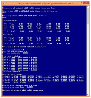
A good way to see where this article is headed and to get an idea of what neural network training with MSO is, is to take a look at the demo program in Figure 1. The goal of the demo program is to use MSO to create a neural network model that predicts a three-class Y-variable for a set of synthetic (programmatically generated) data.
 [Click on image for larger view.]
Figure 1. Neural Network Training Using Multi-Swarm Optimization
[Click on image for larger view.]
Figure 1. Neural Network Training Using Multi-Swarm Optimization
The demo program begins by creating 1,000 random data items where there are four predictor variables (often called features in machine learning terminology). Each feature value is between -10.0 and +10.0, and the 1-of-N encoded Y-value is in the last three columns of the data set.
The 1,000-item data set is randomly split into an 800-item training set used to create the neural network model, and a 200-item test set used to evaluate the accuracy of the model after training. The demo program creates a 4-input, 5-hidden, 3-output neural network classifier and then uses four swarms, each with four particles, to train the classifier. MSO is an iterative process and the maximum number of iterations, maxEpochs, is set to 10,000.
The demo displays the best (smallest) error found by any particle, every 1,000 epochs. A 4-5-3 neural network has (4 * 5) + 5 + (5 * 3) + 3 = 43 weights and biases. After training completed, the 43 best weights and bias values found were (-4.00, -2.57, ... 0.20). Using these weights and bias values, the accuracy of the neural network model was calculated for the training data (91.88 percent correct, which is 735 out of 800) and for the test data (87.50 percent correct, which is 175 out of 200). The accuracy of the model on the test data gives you a rough estimate of how well the model would do if presented with new data that has unknown output values.
This article assumes you have at least intermediate-level programming skills and a solid understanding of the neural network feed-forward mechanism, but does not assume you know anything about MSO. The demo program is coded using C#, but you shouldn't have too much difficulty refactoring the code to another language such as Visual Basic .NET or Python.
The demo code is too long to present here in its entirety, but the complete source code is available in the code download that accompanies this article. The demo code has all normal error checking removed to keep the main ideas as clear as possible and the size of the code small.
Overall Program Structure
The overall program structure, with a few minor edits to save space, is presented in Listing 1. To create the demo, I launched Visual Studio and created a new C# console application named NeuralNetWithMSO. The demo has no significant Microsoft .NET Framework dependencies, so any recent version of Visual Studio will work.
After the template code loaded into the Visual Studio editor, in the Solution Explorer window I renamed the Program.cs file to the more descriptive NeuralNetMultiProgram.cs and Visual Studio automatically renamed class Program for me. At the top of the source code, I deleted all using statements that pointed to unneeded namespaces, leaving just the reference to the top-level System namespace.
Listing 1: Overall Demo Program Structure
using System;
namespace NeuralNetWithMSO
{
  class Program
  {
    static void Main(string[] args)
    {
      Console.WriteLine("Begin NN with multi-swarm demo");

      int numInput = 4; // Number features
      int numHidden = 5;
      int numOutput = 3; // Classes for Y
      int numRows = 1000;
      int seed = 0;

      Console.WriteLine("Generating " + numRows +
        " artificial data items with " + numInput + " features");
      double[][] allData = MakeAllData(numInput, numHidden,
        numOutput, numRows, seed);
      Console.WriteLine("Done");

      Console.WriteLine("Creating train and test matrices");
      double[][] trainData;
      double[][] testData;
      MakeTrainTest(allData, 0.80, seed, out trainData, out testData);
      Console.WriteLine("Done");

      Console.WriteLine("Training data: ");
      ShowData(trainData, 4, 2, true);

      Console.WriteLine("Test data: ");
      ShowData(testData, 3, 2, true);

      Console.WriteLine("Creating a " + numInput + "-" +
        numHidden + "-" +  numOutput + " neural network");
      NeuralNetwork nn =
        new NeuralNetwork(numInput, numHidden, numOutput);

      int numSwarms = 4;
      int numParticles = 4;
      int maxEpochs = 10000;
      Console.WriteLine("Setting numSwarms = " + numSwarms);
      Console.WriteLine("Setting numParticles = " + numParticles);
      Console.WriteLine("Setting maxEpochs = " + maxEpochs);
      Console.WriteLine("Starting training");
      double[] bestWeights =
        nn.Train(trainData, maxEpochs, numSwarms, numParticles);
      Console.WriteLine("Training complete\n");
      Console.WriteLine("Best weights found:");
      ShowVector(bestWeights, 4, 10, true);

      double trainAcc = nn.Accuracy(trainData, bestWeights);
      Console.WriteLine("Accuracy on training data = " +
        trainAcc.ToString("F4"));

      double testAcc = nn.Accuracy(testData, bestWeights);
      Console.WriteLine("Accuracy on test data = " +
        testAcc.ToString("F4"));

      Console.WriteLine("End demo");
      Console.ReadLine();
    } // Main

    static double[][] MakeAllData(int numInput, int numHidden,
      int numOutput, int numRows, int seed) { . . }

    static double HyperTan(double x) { . . }
    static double[] Softmax(double[] oSums) { . . }

    static void MakeTrainTest(double[][] allData, double trainPct,
      int seed, out double[][] trainData,
      out double[][] testData) { . . }

    static void ShowData(double[][] data, int numRows,
      int decimals, bool indices) { . . }

    static void ShowVector(double[] vector, int decimals,
      int lineLen, bool newLine) { . . }

  } // Program

  public class NeuralNetwork
  {
    // data and methods here
    private class Particle { . . }
    private class Swarm { . . }
    private class MultiSwarm { . . }
  }
} // ns
The program class has static helper methods MakeAllData, HyperTan, Softmax, MakeTrainTest, ShowData and ShowVector. All of the neural network logic is contained in a single NeuralNetwork class. The NeuralNetwork class contains nested helper classes Particle, Swarm and MultiSwarm that house the MSO data and logic used during training. These helper classes could've been defined outside of the NeuralNetwork class.
The Main method is obscured by a lot of WriteLine statements, but the key calling statements are quite simple. The synthetic data is generated like so:
int numInput = 4;
int numHidden = 5;
int numOutput = 3;
int numRows = 1000;
int seed = 0;
double[][] allData = MakeAllData(numInput, numHidden,
  numOutput, numRows, seed);
Method MakeAllData creates 43 random weights and bias values between -10.0 and +10.0, then for each data item, random x-values also between -10.0 and +10.0 are generated. Then MakeAllData uses the neural network feed-forward mechanism to generate three numeric output values. These output values will sum to 1.0. The largest output value is encoded as a 1, the other two are encoded as 0. For example, if the three numeric outputs are (0.35, 0.55, 0.10) then the encoded Y-value is (0, 1, 0).
The data is split into training and test sets with these statements:
double[][] trainData;
double[][] testData;
MakeTrainTest(allData, 0.80, seed,
  out trainData, out testData);
The neural network model is created and trained with these statements:
NeuralNetwork nn = new NeuralNetwork(numInput, numHidden,
  numOutput);
int numSwarms = 4;
int numParticles = 4;
int maxEpochs = 10000;
double[] bestWeights = nn.Train(trainData, maxEpochs,
  numSwarms, numParticles);
And the accuracy of the model is calculated with these two statements:
double trainAcc = nn.Accuracy(trainData, bestWeights);
double testAcc = nn.Accuracy(testData, bestWeights);
Understanding the MSO Algorithm
In very high-level pseudo-code, MSO optimization is shown in Listing 2.
Listing 2: Multi-Swarm Optimization in High-Level Pseudo-Code
for-each swarm
  initialize each particle to a random position
end-for

for-each swarm
  for-each particle in swarm
    compute new velocity
    use new velocity to compute new position
    check if position is a new best
    does particle die?
    does particle move to different swarm?
  end-for
end-for

return best position found
The key part of the MSO algorithm is computing a particle's velocity. A velocity is just a set of values that controls to where a particle will move. For example, for a problem with just two x-dimensions, if a particle is at (6.0, 8.0) and the velocity is (-2.0, 1.0), the particle's new position will be at (4.0, 9.0).
Velocity is calculated so that a particle:
- tends to move in its current direction
- tends to move toward its best position found to date
- tends to move toward the best position found by any of its fellow swarm members
- tends to move toward the best position found by any particle in any swarm
In math terms, if x(t) is a particle's position at time t, then a new velocity, v(t+1) is calculated as:
v(t+1) = w * v(t) +
         (c1 * r1) * (p(t) - x(t)) +
         (c2 * r2) * (s(t) - x(t)) +
         (c3 * r3) * (g(t) - x(t))
Term p(t) is the position of the particle's best-known position. Term s(t) is the best position of any particle in the particle's swarm. Term g(t) is the global best position of any particle in any swarm. Term w is a constant called the inertia factor. Terms c1, c2 and c3 are constants that establish a maximum change for each component of the new velocity. Terms r1, r2 and r3 are random values between 0 and 1 that provide a randomization effect to each velocity update.
Suppose a particle is currently at (20.0, 30.0) and its current velocity is (-1.0, -3.0). Also, the best-known position of the particle is (10.0, 12.0), the best-known position of any particle in the swarm is (8.0, 9.0), and the best-known position of any particle in any swarm is (5.0, 6.0). And suppose that constant w has value 0.7, constants c1 and c2 are both 1.4, and constant c3 is 0.4. Finally, suppose random values r1, r2 and r3 are all 0.2.
The new velocity of the particle (with rounding to one decimal) is:
v(t+1) = 0.7 * (-1.0, -3.0) +
         (1.4 * 0.2) * ((10.0, 12.0) - (20.0, 30.0)) +
         (1.4 * 0.2) * ((8.0, 9.0) - (20.0, 30.0)) +
         (0.4 * 0.2) * ((5.0, 6.0) - (20.0, 30.0))

       = 0.7 * (-1.0, -3.0) +
         0.3 * (-10.0, -18.0) +
         0.3 * (-12.0, -21.0) +
         0.1 * (-15.0, -24.0)

       = (-8.8, -16.2)
And so the particle's new position is:
x(t+1) = (20.0, 30.0) + (-8.8, -16.2)
       = (11.2, 13.8)
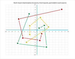
The graph in Figure 2 illustrates the MSO process for a problem with two x-values (just so the process can be displayed in a 2-D graph), three swarms with five particles each, and where the optimal position is at (0, 0). The graph shows how the first particle in each swarm closes in on the optimal position. The spiral motion is characteristic of MSO.
 [Click on image for larger view.]
Figure 2. The Multi-Swarm Optimization Algorithm Illustrated
[Click on image for larger view.]
Figure 2. The Multi-Swarm Optimization Algorithm Illustrated
In the MSO pseudo-code, a particle can die with some low probability. When a particle dies, it's replaced with a new particle at a random position. A particle can immigrate with some low probability. When immigration occurs, a particle is swapped with another particle in a different swarm. The death and immigration mechanisms add an element of randomness to MSO and help prevent the algorithm from getting stuck in a non-optimal solution.
Implementing Neural Network Training Using MSO
The definition of method Train begins as:
public double[] Train(double[][] trainData, int maxEpochs,
      int numSwarms, int numParticles)
{
  int dim = (numInput * numHidden) + numHidden +
    (numHidden * numOutput) + numOutput;
  double minX = -9.9999;
  double maxX = 9.9999;

  MultiSwarm ms = new MultiSwarm(numSwarms, numParticles, dim);
...
The dimension of the problem is the number of weights and bias values to be determined. Variables minX and maxX hold the smallest and largest values for any single value in a Particle object's position array. The NeuralNetwork class contains a nested MultiSwarm class. The MultiSwarm class constructor creates an array-of-arrays of Particle objects, each of which initially has a random position, and a random velocity.
The neural network Error method isn't visible to the MultiSwarm constructor, so method Train supplies the error associated with each particle's position and initializes the best error and associated position:
for (int i = 0; i < numSwarms; ++i)
{
  for (int j = 0; j < numParticles; ++j)
  {
    Particle p = ms.swarms[i].particles[j];
    p.error = MeanSquaredError(trainData, p.position);
    p.bestError = p.error;
    Array.Copy(p.position, p.bestPosition, dim);
…
The nested loops iterate over each swarm, and over each particle in the current swarm. Local variable p is just a convenience reference to refer to the current particle. Next, the current particle is checked to see if it's a swarm-best (smallest error) and if it's a global-best:
…
       if (p.error < ms.swarms[i].bestError) // Swarm best?
    {
      ms.swarms[i].bestError = p.error;
      Array.Copy(p.position, ms.swarms[i].bestPosition, dim);
    }
    if (p.error < ms.bestError) // Global best?
    {
      ms.bestError = p.error;
      Array.Copy(p.position, ms.bestPosition, dim);
    }
  } // j
} // i
The main training loop is prepared like so:
int epoch = 0;
double w = 0.729; // Inertia
double c1 = 1.49445; // Particle
double c2 = 1.49445; // Swarm
double c3 = 0.3645; // Multiswarm
double maxProbDeath = 0.10;
double pImmigrate = 1.0 / maxEpochs;

int[] sequence = new int[numParticles];
for (int i = 0; i < sequence.Length; ++i)
  sequence[i] = i;
The values for constants w, c1 and c2 are the result of some PSO research. Interestingly, compared to many numerical optimization algorithms, PSO and MSO seem to be relatively insensitive to the values used for internal magic constants. There's little available research for the c3 constant that influences the tendency of a particle to move toward the best-known position found to date by any particle in any swarm. The value I use, 0.3645, is half the value of the inertia constant, and has worked well for me in practice.
The array named sequence holds indices of the training data. This array will be scrambled so that in each swarm, particles will be processed in a different order in each iteration of the main training loop.
The main training loop begins:
while (epoch < maxEpochs)
{
  ++epoch;
  for (int i = 0; i < numSwarms; ++i) // each swarm
  {
    Shuffle(sequence);
    for (int pj = 0; pj < numParticles; ++pj) // each particle
    {
      int j = sequence[pj];
      Particle p = ms.swarms[i].particles[j]; // curr particle
…
Knowing when to stop training is one of the most difficult challenges in machine learning. Here, a fixed number, maxEpochs, of iterations is used. Although this approach is simple, there is a risk that you might not train enough. Or you might train too much, which would result in a model that fits the training data extremely well but works poorly on new data. This is called over-fitting. There are many techniques that can be used to combat over-fitting.
Next, the new velocity for the current particle is calculated, as explained earlier (see Listing 3).
Listing 3: Calculating the New Velocity for the Current Particle
for (int k = 0; k < dim; ++k)
{
  double r1 = rnd.NextDouble();
  double r2 = rnd.NextDouble();
  double r3 = rnd.NextDouble();
  p.velocity[k] = (w * p.velocity[k]) +
    (c1 * r1 * (p.bestPosition[k] - p.position[k])) +
    (c2 * r2 * (ms.swarms[i].bestPosition[k] - p.position[k])) +
    (c3 * r3 * (ms.bestPosition[k] - p.position[k]));

  if (p.velocity[k] < minX)
    p.velocity[k] = minX;
  else if (p.velocity[k] > maxX)
    p.velocity[k] = maxX;
}
After the velocity is calculated, each of its component values is checked to see the magnitude is large, and if so, the value is reined back in. This prevents a particle from moving a very great distance in any one iteration. For some machine learning training tasks, eliminating the velocity constraint appears to speed up the training, there are no solid research results in this area of which I'm aware.
Next, the new velocity is used to calculate the current particle's new position and associated error, as shown in Listing 4.
Listing 4: Using the New Velocity to Calculate the Current Particle's New Position and Associated Error
for (int k = 0; k < dim; ++k)
{
  p.position[k] += p.velocity[k];
  if (p.position[k] < minX)
    p.position[k] = minX;
  else if (p.position[k] > maxX)
    p.position[k] = maxX;
}
p.error = Error(trainData, p.position);
if (p.error < p.bestError)
{
  p.bestError = p.error;
  Array.Copy(p.position, p.bestPosition, dim);
}
The current particle is then checked to see if it has moved to a new swarm-best or global-best position:
if (p.error < ms.swarms[i].bestError) // New best for swarm?
{
  ms.swarms[i].bestError = p.error;
  Array.Copy(p.position, ms.swarms[i].bestPosition, dim);
}
if (p.error < ms.bestError) // New global best?
{
  ms.bestError = p.error;
  Array.Copy(p.position, ms.bestPosition, dim);
}
The possibility of death for the current particle comes next:
double p1 = rnd.NextDouble();
double pDeath = (maxProbDeath / maxEpochs) * epoch;
if (p1 < pDeath)
{
  Particle q = new Particle(dim); // A replacement
  q.error = MeanSquaredError(trainData, q.position);
  Array.Copy(q.position, q.bestPosition, dim);
  q.bestError = q.error;
The probability of death varies between 0.0 and maxProbDeath, which was set to 0.10. The probability of death increases linearly as loop counter variable epoch increases. A random value between 0 and 1 is generated, and if this value falls below the death probability threshold, a new replacement for the current particle is generated.
The new particle's position and error must be checked to determine if they're new swarm-best or global-best:
   if (q.error < ms.swarms[i].bestError) // Best swarm error by luck?
  {
    ms.swarms[i].bestError = q.error;
    Array.Copy(q.position, ms.swarms[i].bestPosition, dim);

    if (q.error < ms.bestError) // Best global error?
    {
      ms.bestError = q.error;
      Array.Copy(q.position, ms.bestPosition, dim);
    }
  }

  ms.swarms[i].particles[j] = q; // die!
} // die
Next, the immigration process starts with:
double p2 = rnd.NextDouble();
if (p2 < pImmigrate)
{
  int ii = rnd.Next(0, numSwarms); // rnd swarm
  int jj = rnd.Next(0, numParticles); // rnd particle
  Particle q = ms.swarms[ii].particles[jj];
  ms.swarms[i].particles[j] = q;
  ms.swarms[ii].particles[jj] = p; // The exchange
The immigration mechanism is quite crude. The code selects a random swarm and then a random particle from that swarm, and then swaps the random particle with the current particle. As coded, there's no guarantee that the randomly selected particle will be in a swarm different from the current particle.
Next, because the two particles have new positions and errors, the swarm-best error and position for each of the particles must be checked:
  // p now points to other, q points to curr
  if (q.error < ms.swarms[i].bestError) // Check curr
  {
    ms.swarms[i].bestError = q.error;
    Array.Copy(q.position, ms.swarms[i].bestPosition, dim);
  }
  if (p.error < ms.swarms[ii].bestError) // Check other
  {
    ms.swarms[ii].bestError = p.error;
    Array.Copy(p.position, ms.swarms[ii].bestPosition, dim);
  }
} // Immigrate
Method Train concludes by copying the best position found into the neural network's weights and biases:
…
      } // j - particle
    } // i - swarm
  } // while

  this.SetWeights(ms.bestPosition);
  return ms.bestPosition;
} // Train
Wrapping Up
This article and accompanying code should get you up and running if you want to explore training a neural network using multi-swarm optimization. Based on my experiences, training with MSO tends to give better results than training with back propagation, especially for neural networks with multiple hidden layers (sometimes called deep neural networks). However, MSO is almost always significantly slower than back propagation, and in short, MSO trades off accuracy and performance.