The Data Science Lab
Linear Ridge Regression Using C#
Implementing LRR from scratch is harder than using a library like scikit-learn, but it helps you customize your code, makes it easier to integrate with other systems, and gives you a complete understanding of how LRR works.
The goal of a machine learning regression problem is to predict a single numeric value. For example, you might want to predict the price of a house based on its square footage, number of bedrooms, local tax rate and so on.
There are roughly a dozen major regression techniques, and each technique has several variations. Among the most common techniques are linear regression, linear ridge regression, k-nearest neighbors regression, kernel ridge regression, Gaussian process regression, decision tree regression and neural network regression. This article explains how to implement linear ridge regression from scratch, using the C# language.
Linear ridge regression (LRR) is a relatively simple variation of standard linear regression. However, LRR and standard linear regression are usually considered distinct techniques, in part because they are often applied to different types of problems. LRR is typically used for machine learning scenarios where there is training and test data.
A good way to see where this article is headed is to take a look at the screenshot of a demo program in Figure 1. The demo program uses synthetic data that was generated by a 3-10-1 neural network with random weights. There are three predictor variables that have values between -1.0 and +1.0, and a target variable to predict, which is a value between 0.0 and 1.0. There are 40 training items and 10 test items.
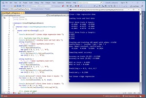 [Click on image for larger view.] Figure 1: Linear Ridge Regression in Action
The demo program creates a linear ridge regression model using the training data. The model uses a parameter named alpha, which is set to 0.05. The alpha value is the "ridge" part of "linear ridge regression." The alpha parameter is used behind the scenes to create L2 regularization, which is a standard machine learning technique to prevent model overfitting. The value of alpha must be determined by trial and error.
After the LRR model is created, it is applied to the training and test data. The model scores 95 percent accuracy on the training data (38 out of 40 correct) and 90 percent accuracy on the test data (9 out of 10 correct). A correct prediction is one that is within 10 percent of the true target value.
The demo program computes and displays the root mean squared error (RMSE) of the model. RMSE is a more granular metric than accuracy, but RMSE is more difficult to interpret. The RMSE on the training data is 0.0209 and 0.0300 on the test data.
The demo program concludes by making a prediction for a new, previously unseen data item x = (0.5, -0.6, 0.7). The predicted y value is 0.2500.
This article assumes you have intermediate or better programming skill but doesn't assume you know anything about linear ridge regression. The demo is implemented using C# but you should be able to refactor the code to a different C-family language if you wish.
The source code for the demo program is too long to be presented in its entirety in this article. The complete code is available in the accompanying file download. The demo code and data are also available online.
Understanding Linear Ridge Regression
A standard linear regression model has the form y = f(x1, x2, . . xn) = w0 + (w1 * x1) + (w2 * x2) + . . + (wn * xn). The xi are the input values. The wi are the coefficients (also called weights). The special w0 value is the constant (also called bias or intercept). For example, if X = (x1, x2, x3) = (0.5, 0.6, 0.2) and W = (w1, w2, w3) = (0.35, -0.45, 0.15) and the bias w0 = 0.65 then the predicted y is 0.65 + (0.35 * 0.5) + (-0.45 * 0.6) + (0.15 * 0.2) = 0.585. Notice that the constant w0 term can be considered a normal coefficient that has a dummy associated input x0 = 1.0.
Simple. But where do the wi values come from? Suppose you have training data that looks like:
x0    x1    x2    x3    y
---------------------------
1.0  -0.5   0.4  -0.9  0.54
1.0   0.3   0.6  -0.3  0.92
1.0  -0.6  -0.7   0.5  0.44
. . .
Notice that a leading column of 1s has been added to the data to act as dummy inputs for the w0 constant term. This is called a design matrix, DX.
Expressed mathematically, the solution for the weights vector w is:
1. DX * w = y
2. DXt * DX * w = DXt * y
3. inv(DXt * DX) * (DXt * DX) * w = inv(DXt * DX) * DXt * y
4. I * w = inv(DXt * DX) * DXt * y
5. w = inv(DXt * DX) * DXt * y
The DX is the design matrix of x values. DXt is the transpose of the design matrix. The * means matrix multiplication. The inv() is matrix inversion. The I represents the identity matrix.
In words, the weight vector is the inverse of the design matrix times its transpose, times the transpose of the design matrix, times the target values. The key point is that if you have training data, there is a closed form solution to compute the model weights.
So far, this is all standard linear regression. But there are two problems. First, the solution for the model weights involves finding the inverse of the DXt * DX matrix. Matrix inversion is quite tricky and can fail for several reasons. Second, because there is likely noise error in the training data, an exact solution for the weights vector often produces weight values that are huge in magnitude, which in turn produces a model that tends to overfit. This means the model predicts very well on the training data, but predicts poorly on new, previously unseen data.
Linear ridge regression solves both problems in a remarkably simple way. A small value, usually called alpha or lambda or noise, is added to the diagonal of the DXt * DX matrix before finding its inverse. The alpha values prevent columns in the DXt * DX matrix from being mathematically correlated, which is the most common cause of failure for matrix inversion. This is called conditioning the matrix. And, although it's not obvious, adding an alpha to the diagonal of the DXt * Dx matrix introduces L2 regularization, which keeps the magnitudes of the weight values small, which in turn discourages model overfitting.
Because LRR adds the same small constant alpha value to each column of the DXt * DX matrix, the predictor data should be normalized to roughly the same scale. The three most common normalization techniques are divide-by-k, min-max and z-score. I recommend divide-by k. For example, if one of the predictor variables is a person's age, you could divide all ages by 100 so that the normalized values are all between 0.0 and 1.0.
Overall Program Structure
I used Visual Studio 2022 (Community Free Edition) for the demo program. I created a new C# console application and checked the "Place solution and project in the same directory" option. I specified .NET version 6.0. I named the project LinearRidgeRegressNumeric. I checked the "Do not use top-level statements" option to avoid the confusing program entry point shortcut syntax.
The demo has no significant .NET dependencies, and any relatively recent version of Visual Studio with .NET (Core) or the older .NET Framework will work fine. You can also use Visual Studio Code if you like.
After the template code loaded into the editor, I right-clicked on file Program.cs in the Solution Explorer window and renamed the file to the more descriptive LinearRidgeRegressNumericProgram.cs. I allowed Visual Studio to automatically rename class Program.
The overall program structure is presented in Listing 1. The Program class houses the Main() method and helper Accuracy() and RootMSE() functions. The LinearRidgeRegress class houses all the linear ridge regression functionality such as the Train() and Predict() methods. The Utils class houses all the matrix helper functions such as MatLoad() to load data into a matrix from a text file, and MatInverse() to find the inverse of a matrix.
Listing 1: Overall Program Structure
using System;
using System.IO;

namespace LinearRidgeRegressNumeric
{
  internal class LinearRidgeRegressNumericProgram
  {
    static void Main(string[] args)
    {
      Console.WriteLine("Linear ridge regression demo ");

      // 1. load data from file to memory
      // 2. create LRR model
      // 3. train model
      // 4. evaluate model
      // 5. use model

      Console.WriteLine("End linear ridge regression ");
      Console.ReadLine();
    } // Main

    static double Accuracy(LinearRidgeRegress model,
      double[][] dataX, double[] dataY,
      double pctClose) { . . }

    static double RootMSE(LinearRidgeRegress model,
      double[][] dataX, double[] dataY) { . . }

  } // Program

  public class LinearRidgeRegress
  {
    public double[]? coeffs;
    public double alpha;

    public LinearRidgeRegress(double alpha) { . . }

    public void Train(double[][] trainX,
      double[] trainY) { . . }

    public double Predict(double[] x) { . . }
  }

  public class Utils
  {
    public static double[][] VecToMat(double[] vec,
      int nRows, int nCols) { . . }

    public static double[][] MatCreate(int rows,
      int cols) { . . }

    public static double[] MatToVec(double[][] m) { . . }

    public static double[][] MatProduct(double[][] matA,
      double[][] matB) { . . }

    public static double[][]
      MatTranspose(double[][] m) { . . }

    public static double[][]
      MatInverse(double[][] m) { . . }

    private static int MatDecompose(double[][] m,
      out double[][] lum, out int[] perm) { . . }

    private static double[] Reduce(double[][] luMatrix,
      double[] b) { . . }

    private static int NumNonCommentLines(string fn,
    string comment) { . . }

    public static double[][] MatLoad(string fn,
      int[] usecols, char sep, string comment) { . . }

    public static double[][]
      MatMakeDesign(double[][] m) { . . }

    public static void MatShow(double[][] m,
      int dec, int wid) { . . }

    public static void VecShow(double[] vec,
      int dec, int wid, bool newLine) { . . }

  } // class Utils
} // ns
The demo program begins by loading the synthetic training data into memory:
Console.WriteLine("Loading train and test data ");
string trainFile =
  "..\\..\\..\\Data\\synthetic_train.txt";
double[][] trainX =
  Utils.MatLoad(trainFile,
  new int[] { 0, 1, 2 }, ',', "#");
double[] trainY =
  Utils.MatToVec(Utils.MatLoad(trainFile,
  new int[] { 3 }, ',', "#"));
The code assumes the data is located in a subdirectory named Data. The MatLoad() utility function specifies that the data is comma delimited and uses the "#" character to identify lines that are comments. The test data is loaded into memory in the same way:
string testFile =
  "..\\..\\..\\Data\\synthetic_test.txt";
double[][] testX =
  Utils.MatLoad(testFile,
  new int[] { 0, 1, 2 }, ',', "#");
double[] testY =
  Utils.MatToVec(Utils.MatLoad(testFile,
  new int[] { 3 }, ',', "#"));
Next, the demo displays the first three test predictor values and target values:
Console.WriteLine("First three train X inputs: ");
for (int i = 0; i < 3; ++i)
  Utils.VecShow(trainX[i], 4, 9, true);

Console.WriteLine("First three train y targets: ");
for (int i = 0; i < 3; ++i)
  Console.WriteLine(trainY[i].ToString("F4"));
In a non-demo scenario you'd probably want to display all training and test data to make sure it was loaded correctly.
The linear ridge regression model is created using the class constructor:
double alpha = 0.05;
Console.WriteLine("Creating and training LRR model" +
  " with alpha = " + alpha.ToString("F3"));
Console.WriteLine("Coefficients = " +
  " inv(DXt * DX) * DXt * Y ");
LinearRidgeRegress lrrModel =
  new LinearRidgeRegress(alpha);
The LRR constructor accepts the alpha parameter. The value of alpha must be determined by experimentation. Larger values of alpha retard the magnitudes of the model coefficients, which improves generalizability, but at the expense of accuracy.
The model is trained like so:
lrrModel.Train(trainX, trainY);
Console.WriteLine("Done. Model constant," +
  " coefficients = ");
Utils.VecShow(lrrModel.coeffs, 4, 9, true);
Behind the scenes, the Train() method uses the algorithm explained in the previous section. After the model has been trained, it is evaluated:
Console.WriteLine("Computing model accuracy ");
double accTrain =
  Accuracy(lrrModel, trainX, trainY, 0.10);
Console.WriteLine("Accuracy on train (0.10) = "
  + accTrain.ToString("F4"));
Because there's no inherent definition of regression accuracy, it's necessary to implement a program-defined function. How close a predicted value must be to the true value in order to be considered a correct prediction will vary from problem to problem. The test accuracy is computed in the same way:
double accTest =
  Accuracy(lrrModel, testX, testY, 0.10);
Console.WriteLine("Accuracy on test (0.10) = " +
  accTest.ToString("F4"));
The demo computes the root mean squared error of the model on the training and test data. Because the RMSE values on the training data (0.0209) and test data (0.0300) are similar, there's reason to believe that the model does not seriously overfit.
The demo concludes by using the trained model to predict for X = (0.5, -0.6, 0.7) using these statements:
Console.WriteLine("Predicting x = 0.5, -0.6, 0.7 ");
double[] x = new double[] { 0.5, -0.6, 0.7 };
double predY = lrrModel.Predict(x);
Console.WriteLine("\Predicted y = " +
  predY.ToString("F4"));
The Predict() method expects a single vector of predictor values. A common design alternative is to implement Predict() to accept an array of vectors, which is equivalent to a matrix. Notice that Predict() is not expecting a leading dummy 1.0 value to act as input for the model constant / bias.
The Predict Method
The Predict() method is simple. The method assumes that the constant / bias is located at index [0] of the coeffs vector. Therefore, input x[i] is associated with coeffs[i+1].
public double Predict(double[] x)
{
  // constant at coeffs[0]
  double sum = 0.0;
  int n = x.Length;  // number predictors
  for (int i = 0; i < n; ++i)
    sum += x[i] * this.coeffs[i + 1];

  sum += this.coeffs[0];  // add the constant
  return sum;
}
In a non-demo scenario you might want to add normal error checking, such as making sure that the length of the input x vector is equal to 1 less than the length of the coeffs vector.
The Train Method
The Train() method, shown in Listing 1, is short but dense because most of the work is farmed out to matrix functions in the Utils class. The training code starts with:
public void Train(double[][] trainX, double[] trainY)
{
  double[][] DX =
    Utils.MatMakeDesign(trainX);  // add 1s column
. . .
The MatMakeDesign() function programmatically adds a leading column of 1s to act as inputs for the constant / bias term. An alternative approach is to physically add a leading column of 1s to the training data.
Next, the DXt * DX matrix is computed:
  // coeffs = inv(DXt * DX) * DXt * Y
  double[][] a = Utils.MatTranspose(DX);
  double[][] b = Utils.MatProduct(a, DX);
Breaking the code down into small intermediate statements is not necessary but makes the code easier to debug, compared to a single statement like double[][] b = Utils.MatProduct(Utils.MatTranspose(DX), DX).
At this point the alpha / noise value is added to the diagonal of the DXt * DX matrix:
  for (int i = 0; i < b.Length; ++i)
   b[i][i] += this.alpha;
If alpha = 0, then no matrix conditioning or L2 regularization is applied and linear ridge regression reduces to standard linear regression.
The Train() method concludes with:
. . .
  double[][] c = Utils.MatInverse(b);
  double[][] d = Utils.MatProduct(c, a);
  double[][] Y = Utils.VecToMat(trainY, DX.Length, 1);
  double[][] e = Utils.MatProduct(d, Y);
  this.coeffs = Utils.MatToVec(e);
}
The utility MatInverse() function uses Crout's decomposition algorithm. A significantly different approach is to avoid computing a matrix inverse directly and use an indirect technique called QR decomposition. The QR decomposition approach is used by many machine learning libraries because it is slightly more efficient than using matrix inverse. However, using matrix inverse is a much cleaner design in my opinion.
Notice that in order to multiply the vector of target y values in trainY times the inverse, the target y values must be converted from a one-dimensional vector to a two-dimensional matrix using the VecToMat() function. Then after the matrix multiplication, the resulting matrix must be converted back to a vector using the MatToVec() function. Details like this can be a major source of bugs during development.
Because the linear ridge regression training algorithm presented in this article inverts a matrix, the technique doesn't scale to problems with huge amounts of training data. In such situations, it is possible to use stochastic gradient descent (SGD) to estimate model coefficients and constant / bias. You can see an example of SGD training on the data used in my article, "Linear Ridge Regression from Scratch Using C# with Stochastic Gradient Descent."
Wrapping Up
To recap, linear ridge regression is essentially standard linear regression with L2 regularization added to prevent huge model coefficient values that can cause model overfitting. The weakness of linear ridge regression compared to more powerful techniques such as kernel ridge regression and neural network regression is that LRR assumes that data is linear. Even when an LRR model doesn't predict well, LRR is still useful to establish baseline results. The main advantage of LRR is simplicity.
The demo program uses strictly numeric predictor variables. LRR can handle categorical data such as a predictor variable of color with possible values red, blue and green. Each categorical value can be one-hot encoded, for example red = (1, 0, 0), blue = (0, 1, 0) and green = (0, 0, 1). In standard linear regression it's usually a mistake to use one-hot encoding because the resulting columns are mathematically correlated, which causes matrix inversion to fail. Standard linear regression uses a somewhat ugly technique (in my opinion) called dummy coding for categorical predictor variables.
Implementing LRR from scratch requires more effort than using a library such as scikit-learn. But implementing from scratch allows you to customize your code, makes it easier to integrate with other systems, and gives you a complete understanding of how LRR works.