Neural Network Lab

Coding Neural Network Back-Propagation Using C#

Back-Propagation is the most common algorithm for training neural networks. Here's how to implement it in C#.

• By James McCaffrey
• 04/14/2015

Back-propagation is the most common algorithm used to train neural networks. There are many ways that back-propagation can be implemented. This article presents a code implementation, using C#, which closely mirrors the terminology and explanation of back-propagation given in the Wikipedia entry on the topic.

You can think of a neural network as a complex mathematical function that accepts numeric inputs and generates numeric outputs. The values of the outputs are determined by the input values, the number of so-called hidden processing nodes, the hidden and output layer activation functions, and a set of weights and bias values.

A fully connected neural network with m inputs, h hidden nodes, and n outputs has (m * h) + h + (h * n) + n weights and biases. For example, a neural network with 4 inputs, 5 hidden nodes, and 3 outputs has (4 * 5) + 5 + (5 * 3) + 3 = 43 weights and biases. Training a neural network is the process of finding values for the weights and biases so that, for a set of training data with known input and output values, the computed outputs of the network closely match the known outputs.

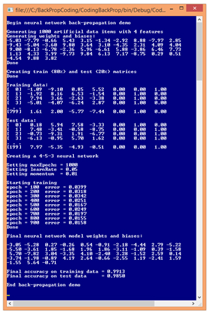
The best way to see where this article is headed is to examine the demo program in Figure 1. The demo program begins by generating 1,000 synthetic data items. Each data item has four input values and three output values. For example, one of the synthetic data items is:

-1.09  -9.10  0.85  5.52  0  0  1

The four input values are all between -10.0 and +10.0 and correspond to predictor values that have been normalized so that values below zero are smaller than average, and values above zero are greater than average. The three output values correspond to a variable to predict that can take on one of three categorical values. For example, you might want to predict the political leaning of a person: conservative, moderate or liberal. Using 1-of-N encoding, conservative is (1, 0, 0), moderate is (0, 1, 0), and liberal is (0, 0, 1). So, for the example data item, if the predictor variables are age, income, education, and debt, the data item represents a person who is younger than average, has much lower income than average, is somewhat more educated than average, and has higher debt than average. The person has a liberal political view.

After the 1,000 data items were generated, the demo program split the data randomly, into an 8,000-item training set and a 2,000-item test set. The training set is used to create the neural network model, and the test set is used to estimate the accuracy of the model.

After the data was split, the demo program instantiated a neural network with five hidden nodes. The number of hidden nodes is arbitrary and in realistic scenarios must be determined by trial and error. Next, the demo sets the values of the back-propagation parameters. The maximum number of training iterations, maxEpochs, was set to 1,000. The learning rate, learnRate, controls how fast training works and was set to 0.05. The momentum rate, momentum, is an optional parameter to increase the speed of training and was set to 0.01. Training parameter values must be determined by trial and error.

During training, the demo program calculated and printed the mean squared error, every 100 epochs. In general, the error decreased over time, but there were a few jumps in error. This is typical behavior when using back-propagation. When training finished, the demo displayed the values of the 43 weights and biases found. These values, along with the number of hidden nodes, essentially define the neural network model.

The demo concluded by using the weights and bias values to calculate the predictive accuracy of the model on the training data (99.13 percent, or 7,930 correct out of 8,000) and on the test data (98.50 percent, or 1,970 correct out of 2,000). The demo didn't use the resulting model to make a prediction. For example, if the model is fed input values (1.0, 2.0, 3.0, 4.0), the predicted output is (0, 1, 0), which corresponds to a political moderate.

This article assumes you have at least intermediate level developer skills and a basic understanding of neural networks but does not assume you are an expert using the back-propagation algorithm. The demo program is too long to present in its entirety here, but complete source code is available in the download that accompanies this article. All normal error checking has been removed to keep the main ideas as clear as possible.

The Demo Program
To create the demo program, I launched Visual Studio, selected the C# console application program template, and named the project CodingBackProp. The demo has no significant Microsoft .NET Framework version dependencies, so any relatively recent version of Visual Studio should work. After the template code loaded, in the Solution Explorer window I renamed file Program.cs to BackPropProgram.cs and Visual Studio automatically renamed class Program for me.

The overall structure of the demo program is presented in Listing 1. I removed unneeded using statements that were generated by the Visual Studio console application template, leaving just the one reference to the top-level System namespace.

using System;
namespace CodingBackProp
{
  class BackPropProgram
  {
    static void Main(string[] args)
    {
      Console.WriteLine("Begin back-propagation demo");
      ...
      Console.WriteLine("End back-propagation demo");
      Console.ReadLine();
    }

    public static void ShowMatrix(double[][] matrix,
      int numRows, int decimals, bool indices) { . . }
    
    public static void ShowVector(double[] vector,
      int decimals, int lineLen, bool newLine) { . . }
    
    static double[][] MakeAllData(int numInput,
      int numHidden, int numOutput, int numRows,
      int seed) { . . }
    
    static void SplitTrainTest(double[][] allData,
      double trainPct, int seed, out double[][] trainData,
      out double[][] testData) { . . }
  } // Program

  public class NeuralNetwork
  {
    private int numInput;
    private int numHidden;
    private int numOutput;

    private double[] inputs;
    private double[][] ihWeights;
    private double[] hBiases;
    private double[] hOutputs;

    private double[][] hoWeights;
    private double[] oBiases;
    private double[] outputs;

    private Random rnd;

    public NeuralNetwork(int numInput, int numHidden,
      int numOutput) { . . }
    
    private static double[][] MakeMatrix(int rows,
      int cols, double v) { . . }
    
    private void InitializeWeights() { . . }
    
    public void SetWeights(double[] weights) { . . }
    public double[] GetWeights() { . . }
    
    public double[] ComputeOutputs(double[] xValues) { . . }
    private static double HyperTan(double x) { . . }
    private static double[] Softmax(double[] oSums) { . . }
    
    public double[] Train(double[][] trainData,
      int maxEpochs, double learnRate,
      double momentum) { . . }
    
    private void Shuffle(int[] sequence) { . . }
    private double Error(double[][] trainData) { . . }
    
    public double Accuracy(double[][] testData) { . . }
    private static int MaxIndex(double[] vector) { . . }
  } // NeuralNetwork
} // ns

All the control logic is in the Main method and all the classification logic is in a program-defined NeuralNetwork class. Helper method MakeAllData generates a synthetic data set. Method SplitTrainTest splits the synthetic data into training and test sets. Methods ShowData and ShowVector are used to display training and test data, and neural network weights.

The Main method (with a few minor edits to save space) begins by preparing to create the synthetic data:

static void Main(string[] args)
{
  Console.WriteLine("Begin back-propagation demo");
  int numInput = 4; // number features
  int numHidden = 5;
  int numOutput = 3; // number of classes for Y
  int numRows = 1000;
  int seed = 1; // gives nice demo

Next, the synthetic data is created:

Console.WriteLine("\nGenerating " + numRows +
  " artificial data items with " + numInput + " features");
double[][] allData = MakeAllData(numInput, numHidden,
  numOutput, numRows, seed);
Console.WriteLine("Done");

To create the 1,000-item synthetic data set, helper method MakeAllData creates a local neural network with random weights and bias values. Then, random input values are generated, the output is computed by the local neural network using the random weights and bias values, and then output is converted to 1-of-N format.

Next, the demo program splits the synthetic data into training and test sets using these statements:

Console.WriteLine("Creating train and test matrices");
double[][] trainData;
double[][] testData;
SplitTrainTest(allData, 0.80, seed,
  out trainData, out testData);
Console.WriteLine("Done");
Console.WriteLine("Training data:");
ShowMatrix(trainData, 4, 2, true);
Console.WriteLine("Test data:");
ShowMatrix(testData, 4, 2, true);

Next, the neural network is instantiated like so:

Console.WriteLine("Creating a " +  numInput + "-" +
  numHidden + "-" + numOutput + " neural network");
NeuralNetwork nn = new NeuralNetwork(numInput,
  numHidden, numOutput);

The neural network has four inputs (one for each feature) and three outputs (because the Y variable can be one of three categorical values). The choice of five hidden processing units for the neural network is the same as the number of hidden units used to generate the synthetic data, but finding a good number of hidden units in a realistic scenario requires trial and error. Next, the back-propagation parameter values are assigned with these statements:

int maxEpochs = 1000;
double learnRate = 0.05;
double momentum = 0.01;
Console.WriteLine("Setting maxEpochs = " +
  maxEpochs);
Console.WriteLine("Setting learnRate = " +
  learnRate.ToString("F2"));
Console.WriteLine("Setting momentum  = " +
  momentum.ToString("F2"));

Determining when to stop neural network training is a difficult problem. Here, using 1,000 iterations was arbitrary. The learning rate controls how much each weight and bias value can change in each update step. Larger values increase the speed of training at the risk of overshooting optimal weight values. The momentum rate helps prevent training from getting stuck with local, non-optimal weight values and also prevents oscillation where training never converges to stable values.

Training using back-propagation is accomplished with these statements:

Console.WriteLine("Starting training");
double[] weights = nn.Train(trainData, maxEpochs,
  learnRate, momentum);
Console.WriteLine("Done");
Console.WriteLine("Final weights and biases: ");
ShowVector(weights, 2, 10, true);

The Train method stores the best weights and bias values found internally in the NeuralNetwork object, and also returns those values, serialized into a single result array. In a production environment you would likely save the model weights and bias values to a text file so they could be retrieved later, if necessary.

The demo program concludes by calculating the prediction accuracy of the neural network model:

... 
  double trainAcc = nn.Accuracy(trainData);
  Console.WriteLine("Final accuracy on train data = " +
    trainAcc.ToString("F4"));
  double testAcc = nn.Accuracy(testData);
  Console.WriteLine("Final accuracy on test data = " +
    testAcc.ToString("F4"));
  Console.WriteLine("End back-propagation demo");
  Console.ReadLine();
} // Main

The accuracy of the model on the test data gives you a very rough estimate of how accurate the model will be when presented with new data that has unknown output values. The accuracy of the model on the training data is useful to determine if model over-fitting has occurred. If the prediction accuracy of the model on the training data is significantly greater than the accuracy on the test data, then there's a strong likelihood that over-fitting has occurred and re-training with new parameter values is necessary.

Implementing Back-Propagation Training
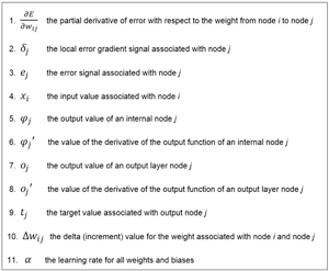
In many areas of computer science, Wikipedia articles have become de facto standard references. This is somewhat true for the neural network back-propagation algorithm. A major hurdle for many software engineers when trying to understand back-propagation, is the Greek alphabet soup of symbols used. Figure 2 presents 11 major symbols used in the Wikipedia explanation of back-propagation. Bear with me here; back-propagation is a complex algorithm but once you see the code implementation, understanding these symbols isn't quite as difficult as it might first appear.

The definition of the back-propagation training method begins by allocating space for gradient values:

public double[] Train(double[][] trainData,
  int maxEpochs, double learnRate, double momentum)
{
  double[][] hoGrads = MakeMatrix(numHidden,
    numOutput, 0.0); // hidden-to-output weight gradients
  double[] obGrads = new double[numOutput];
  double[][] ihGrads = MakeMatrix(numInput,
    numHidden, 0.0);  // input-to-hidden weight gradients
  double[] hbGrads = new double[numHidden];
...

Back-propagation is based on calculus partial derivatives. Each weight and bias value has an associated partial derivative. You can think of a partial derivative as a value that contains information about how much, and in what direction, a weight value must be adjusted to reduce error. The collection of all partial derivatives is called a gradient. However, for simplicity, each partial derivative is commonly just called a gradient.

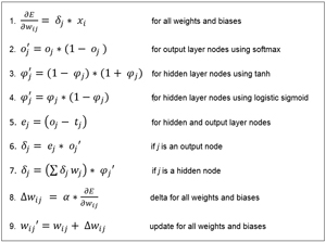
The key math equations of back-propagation are presented in Figure 3. These equations can be intimidating. But interestingly, even for my colleagues who are math guys, many feel that the actual code is easier to understand than the equations.

If you look at the equations in Figure 3 (and your head doesn't explode), you'll see that the weight update (equation 9) is the goal. It involves a weight delta (symbol 10). Calculating the delta (equation 8) uses the learning rate (symbol 11) and the gradients (symbol 1). In code, the values of each of these gradients are stored in hoGrads (hidden-to-output weights), obGrads (output biases), ioGrads (input-to-hidden weights), and hbGrads (hidden biases).

Next, storage arrays for the output and hidden layer local error gradient signals (symbol 2) are allocated:

double[] oSignals = new double[numOutput];
double[] hSignals = new double[numHidden];

Unlike most of the other variables in back-propagation, this variable doesn't seem to have a consistently used standard name, and Wikipedia uses the symbol, which is lowercase Greek delta, without explicitly naming it. I call it the local error gradient signal, or just signal. Note, however, that the similar terms "error signal" and "gradient" have different uses and meanings in back-propagation.

The momentum term is optional, but it is almost always used with back-propagation. Momentum requires the values of the weight and bias deltas (symbol 10) from the previous training iteration. Storage for these previous iteration delta values is allocated like so:

double[][] ihPrevWeightsDelta = MakeMatrix(numInput,
  numHidden, 0.0);
double[] hPrevBiasesDelta = new double[numHidden];
double[][] hoPrevWeightsDelta = MakeMatrix(numHidden,
  numOutput, 0.0);
double[] oPrevBiasesDelta = new double[numOutput];

The main training loop is prepared with these statements:

int epoch = 0;
double[] xValues = new double[numInput];
double[] tValues = new double[numOutput];
double derivative = 0.0;
double errorSignal = 0.0;
int errInterval = maxEpochs / 10;

Variable epoch is the loop counter variable. Array xValues holds the input values from the training data. Array tValues holds the target values from the training data. Variable derivative corresponds to symbols 6 and 8 in Figure 2. Variable errorSignal corresponds to symbol 3. Variable errInterval controls how often to compute and display the current error during training. Before the training loop starts, an array that holds the indices of the training data is created:

int[] sequence = new int[trainData.Length];
for (int i = 0; i < sequence.Length; ++i)
  sequence[i] = i;

During training, it's important to present the training data in a different, random order each time through the training loop. The sequence array will be shuffled and used to determine the order in which training items will be processed. Next, method Train begins the main training loop:

while (epoch < maxEpochs)
{
  ++epoch;
  if (epoch % errInterval == 0 && epoch < maxEpochs)
  {
    double trainErr = Error(trainData);
    Console.WriteLine("epoch = " + epoch +
      " error = " + trainErr.ToString("F4"));
  }
  Shuffle(sequence);
...

Calculating the mean squared error is an expensive operation because all training items must be used in the computation. However, there's a lot that can go wrong during training so it's highly advisable to monitor error. Helper method Shuffle scrambles the indices stored in the sequence array using the Fisher-Yates algorithm. Next, each training item is processed:

for (int ii = 0; ii < trainData.Length; ++ii)
{
  int idx = sequence[ii];
  Array.Copy(trainData[idx], xValues, numInput);
  Array.Copy(trainData[idx], numInput, tValues,
    0, numOutput);
  ComputeOutputs(xValues); 
...

The input and target values are pulled from the current training item. The input values are fed to method ComputeOutputs, which does just that, storing the output values internally. Note that the explicit return value array from ComputeOutputs is ignored. Next, the output node signals (equation 6) are computed:

for (int k = 0; k < numOutput; ++k)
{
  errorSignal = tValues[k] - outputs[k];
  derivative = (1 - outputs[k]) * outputs[k];
  oSignals[k] = errorSignal * derivative;
}

The error signal (equation 5) can be computed as either output minus target, or target minus output. The Wikipedia article uses output minus target which results in the weight deltas being subtracted from current weight values. Most other references prefer the target minus output version, which results in weight deltas being added to current weight values (as shown in equation 9).

The Wikipedia entry glosses over the fact that the output derivative term depends on what activation function is used. Here, the derivative is computed assuming that output layer nodes use softmax activation, which is a form of the logistic sigmoid function. In the unlikely situation that you use a different activation function, you'd have to change this part of the code.

After the output node signals have been computed, they are used to compute the hidden-to-output weight and output bias gradients:

for (int j = 0; j < numHidden; ++j)
  for (int k = 0; k < numOutput; ++k)
    hoGrads[j][k] = oSignals[k] * hOutputs[j];
 
for (int k = 0; k < numOutput; ++k)
  obGrads[k] = oSignals[k] * 1.0;

Notice the dummy 1.0 input value associated with the output bias gradients. This was used just to illustrate the similarity between hidden-to-output weights, where the associated input value comes from hidden layer node local output values, and output node biases, which have a dummy, constant, input value of 1.0. Next, the hidden node signals are calculated:

for (int j = 0; j < numHidden; ++j)
{
  derivative = (1 + hOutputs[j]) * (1 - hOutputs[j]); //tanh
  double sum = 0.0; 
  for (int k = 0; k < numOutput; ++k) {
    sum += oSignals[k] * hoWeights[j][k]; 
  }
  hSignals[j] = derivative * sum; 
}

These calculations implement equation 7 and are the heart of the back-propagation algorithm. They're not at all obvious. The Wikipedia entry explains the beautiful, but complicated math, which gives equation 7. The Wikipedia entry assumes the logistic sigmoid function is used for hidden layer node activation. I much prefer using the hyperbolic tangent function (tanh) and the value of the derivative variable corresponds to tanh. Notice the calculations of the hidden node signals require the values of the output node signals, essentially working backward. This is why back-propagation is named what it is.

Next, the input-to-hidden weight gradients and the hidden bias gradients are calculated:

for (int i = 0; i < numInput; ++i)
  for (int j = 0; j < numHidden; ++j)
    ihGrads[i][j] = hSignals[j] * inputs[i];

for (int j = 0; j < numHidden; ++j)
  hbGrads[j] = hSignals[j] * 1.0;

As before, the dummy 1.0 input value used for the bias gradients can be dropped if you wish. After all gradients have been calculated and stored, method Train updates all weights and bias values, using the gradients. Unlike gradients, where output gradients must be calculated before hidden gradients, weights and biases can be updated in any order. First, the input-to-hidden weights are updated:

for (int i = 0; i < numInput; ++i)
{
  for (int j = 0; j < numHidden; ++j)
  {
    double delta = ihGrads[i][j] * learnRate;
    ihWeights[i][j] += delta;
    ihWeights[i][j] += ihPrevWeightsDelta[i][j] *
                         momentum;
    ihPrevWeightsDelta[i][j] = delta; // save
  }
}

Here, the statement computing the value of variable delta corresponds to equation 8 in Figure 3. That delta value is saved for use in the next iteration to implement the momentum mechanism. Notice that all weights and bias values are updated after the gradients have been calculated for a single training data item. In principle, gradients should be calculated by accumulating error signals over all training items. But updating weights and biases after each training data item essentially estimates the overall gradients and is more efficient. This approach is usually called "online" or "stochastic" training. The alternative is usually called "batch" training.

Next, hidden node biases are updated:

for (int j = 0; j < numHidden; ++j)
{
  double delta = hbGrads[j] * learnRate;
  hBiases[j] += delta;
  hBiases[j] += hPrevBiasesDelta[j] * momentum;
  hPrevBiasesDelta[j] = delta;
}

Next, hidden-to-output weights are updated:

for (int j = 0; j < numHidden; ++j)
{
  for (int k = 0; k < numOutput; ++k)
  {
    double delta = hoGrads[j][k] * learnRate;
    hoWeights[j][k] += delta;
    hoWeights[j][k] += hoPrevWeightsDelta[j][k] *
                         momentum;
    hoPrevWeightsDelta[j][k] = delta;
  }
}

The each-data loop and main training loop finish after updating the output node biases:

...
    for (int k = 0; k < numOutput; ++k)
    {
      double delta = obGrads[k] * learnRate;
      oBiases[k] += delta;
      oBiases[k] += oPrevBiasesDelta[k] * momentum;
      oPrevBiasesDelta[k] = delta;
    }
  } // Each training item
} // While

At this point, the best weights and bias values are stored in the neural network object. Method Train concludes by fetching those values and returning them:

  ...
  double[] bestWts = GetWeights();
  return bestWts;
} // Train

Here, a serialized copy of the internal weights and bias values is created using class method GetWeights. An alternative is to refactor method Train to return void, and then call GetWeights as needed after training.

Wrapping Up
There are several ways you can modify the back-propagation code presented in this article. The version of back-propagation presented here is based on a mathematical assumption about how training error is computed. Specifically, the equations in Figure 3 assume that the goal of training is to find weights and bias values that minimize mean squared error between computed and target output values. There is an alternative form of error, called cross entropy error, which leads to a slightly different version of back-propagation.

Another modification is to use weight decay, also called regularization. The idea here is to use a form of error that penalizes large weight values, which in turn helps prevent model over-fitting where the model predicts very well on the training data, but predicts poorly when presented with new data.

• Get Code Download