The Data Science Lab
Chi-Square Tests Using R
R is the perfect language for creating a variety of chi-square tests, which are used to perform statistical analyses of counts of data. Here's how, with some sample code.
A chi-square test (also called chi-squared test) is a common statistical technique used when you have data that consists of counts in categories. For example, you might have counts of the number of HTTP requests a server gets in each hour during a day, or you might have counts of the number of employees in each job category at your company.
There are several kinds of chi-square tests. The three most common forms are a test for equal counts, a test for counts given specified probabilities, and a test for independence of two factors. In this article I'll show you how to write R language programs (technically scripts because R is interpreted) to perform each of the three basic chi-square tests.
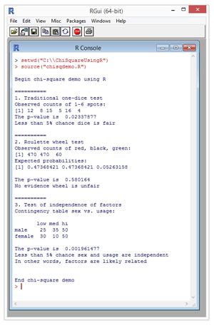
A good way to see where this article is headed is to take a look at a screenshot of a demo program in Figure 1. The demo program is named chisqdemo.R and is running in the R Console shell in the RGui program. The R language system is open source and you can find a simple self-extracting installation executable for Windows systems here.
 [Click on image for larger view.]
Figure 1. Chi-Square Tests Using R
[Click on image for larger view.]
Figure 1. Chi-Square Tests Using R
To execute the demo R program, I first used the setwd (set working directory) command to point to the location of the program. Then I used the source command to run the program.
The first example in the demo tests whether a single dice (OK, I know it's a "die" but that just doesn't sound right) is fair or not. You roll the dice 60 times. Because there are six possible results on each roll, if the dice is fair you'd expect to get a count of about 10 for each of the possible results.
The demo displays the number of times each result actually occurred, then behind the scenes, a chi-square test for equal counts is performed. The results of the test suggest that the dice is not fair. Notice that a six-spot occurred only four times. It's unlikely that you'll be analyzing rolls of a dice at work but gambling examples are traditional when explaining chi-square tests and they easily generalize to useful problems.
The second example tests if a roulette wheel is fair or not. An American-style roulette wheel has 38 total numbers. There are 18 red numbers, 18 black numbers, and two green numbers (0 and 00). Therefore, if you play the wheel many times you'd expect to get about 18/38 = 47% red numbers, 18/38 = 47% black numbers, and 2/38 = 5% green numbers. The demo program performs a chi-square test and concludes that the observed counts are close enough to the expected counts to suggest there's no evidence the wheel is unfair.
The third example tests if, in a group of 200 people, sex (male or female) is independent of the usage (low, medium, high) of some sort of resource like a Web site or tool. The demo chi-square test concludes that the observed counts of data suggest that the two factors, sex and usage, are not independent and, therefore, are likely related to each other in some way.
Testing for Equal Counts
I used Notepad to create the demo program. There are several fancy R editors you can use but any simple text editor will work fine. The complete source code for the demo is presented in Listing 1 and you can also get the code from the download that accompanies this article.
Listing 1: Chi-Square Test Demo Program
# chisqdemo.R
# demonstrate chi-square tests using R

cat("\nBegin chi-square demo using R\n\n")

cat("==========\n")
cat("1. Traditional one-dice test\n")
obs <- c(12, 8, 15, 5, 16, 4)
cat("Observed counts of 1-6 spots: \n")
print(obs)
m <- chisq.test(obs)
cat("The p-value is ", m$p.value, "\n")
if (m$p.value < 0.05) {
cat("Less than 5% chance dice is fair\n\n")
} else {
  cat("No evidence dice is unfair\n\n")
}

cat("==========\n")
cat("2. Roulette wheel test\n")
obs <- c(470, 470, 60)
cat("Observed counts of red, black, green: \n")
print(obs)
probs <- array(0.0, 3) # red, black, green
probs[1] <- 18/38
probs[2] <- 18/38
probs[3] <- 2/38
cat("Expected probabilities: \n")
print(probs)
m <- chisq.test(obs, p=probs)
cat("\nThe p-value is ", m$p.value, "\n")
if (m$p.value < 0.05) {
  cat("Less than 5% chance wheel is fair\n\n")
} else {
  cat("No evidence wheel is unfair\n\n")
}

cat("==========\n")
cat("3. Test of independence of factors\n")
low <- c(25, 30)
med <- c(35, 10)
hi  <- c(50, 50)
dframe <- data.frame(low, med, hi)
rownames(dframe) <- c("male", "female")
cat("Contingency table sex vs. usage: \n\n")
print(dframe)
m <- chisq.test(dframe)
cat("\nThe p-value is ", m$p.value, "\n")
if (m$p.value < 0.05) {
  cat("Less than 5% chance sex and usage are independent\n")
  cat("In other words, factors are likely related\n\n")
} else {
  cat("No evidence sex and usage are independent\n")
  cat("In other words, factors are likely not related\n\n")
}

cat("\nEnd chi-square demo\n")
The first three statements in the demo program are:
# chisqdemo.R
# demonstrate chi-square tests using R
cat("\nBegin chi-square demo using R\n\n")
The "#" character begins an R comment. The cat function is used to send messages to output. The R language is closely related to C, so much of the syntax should look familiar to you. The next few statements are:
cat("1. Traditional one-dice test\n")
obs <- c(12, 8, 15, 5, 16, 4)
cat("Observed counts of 1-6 spots: \n")
print(obs)
The array named obs holds the observed counts of each of the six possible outcomes. So a 1-spot was observed 12 times, a 2-spot was observed eight times, and so on. The tersely named c function creates an array/vector using the supplied values. I typically use the cat function to display messages and the print function to display R objects.
The demo performs a chi-square test for equal counts like so:
m <- chisq.test(obs)
This means, "Do a chi-square test for equal counts using the values in array obs and store the results into an object named m (model)." In R you can use either "<-" or "=" for assignment.
Next, the demo displays the test result p-value:
cat("The p-value is ", m$p.value, "\n")
In R the "$" character is used to specify a field in an object. The variable named p.value is one of the fields in object m. I determined its name by looking at the R documentation for the chisq.test function. Note that in most languages the underscore character is used to make variable names more readable but in R the period character is often used.
The demo then interprets the results of the chi-square test:
if (m$p.value < 0.05) {
  cat("Less than 5% chance dice is fair\n\n")
} else {
  cat("No evidence dice is unfair\n\n")
}
The p-value ("probability value") is the probability that the observed counts could've occurred if the dice was in fact fair and all outcomes were therefore equally likely. Here, the p-value is 0.0234, which is a small value. In statistics, small p-values are usually defined to be 0.05 or 0.01. Put another way, if you do a chi-square test for equal counts (also called a test for a uniform distribution) and the resulting p-value is less than 0.05, you conclude that there seems to be evidence that the counts are not equal. If the resulting p-value is greater than 0.05, you conclude there's insufficient evidence that the counts aren't equal.
Testing for Counts with Specified Probabilities
The second test in the demo program begins with these statements:
cat("2. Roulette wheel test\n")
obs <- c(470, 470, 60)
cat("Observed counts of red, black, green: \n")
print(obs)
Notice that the array named obs is being reused. Here, there are a total of 470 + 470 + 60 = 1,000 spins of the wheel. Next, the probabilities of each of the three possible outcomes are set up in an array named probs:
probs <- array(0.0, 3) # red, black, green
probs[1] <- 18/38
probs[2] <- 18/38
probs[3] <- 2/38
The array function in R is overloaded. The call here sets up an array with 3 cells where each cell value is 0.0. Notice that arrays in R use 1-based indexing rather than 0-based indexing as in almost all other languages. Also, in R numeric types are real by default rather than integer so 18/38 = 0.47 and not 0 as you'd get in a language like C#. The demo could have set up the probs array like so:
probs <- c(18/38, 18/38, 2/38)
I used the longer technique just to illustrate the array function. After displaying the values in the probs array using the print function, the demo performs a chi-square test for counts with specified probabilities:
m <- chisq.test(obs, p=probs)
cat("\nThe p-value is ", m$p.value, "\n")
The R chisq.test function has many optional parameters. If no probability array is passed to chisq.test, the function does a test for equal counts. Notice that R can use named-parameter calls.
Next, the demo interprets the results of the chi-square test:
if (m$p.value < 0.05) {
  cat("Less than 5% chance wheel is fair\n\n")
} else {
  cat("No evidence wheel is unfair\n\n")
}
As with the test for equal counts, if the resulting p-value is small, where the value for small is arbitrary but usually 0.05 or 0.01, then you conclude that the observed counts are unlikely to have occurred given the specified probabilities. If the p-value isn't small, you conclude there's not enough evidence to suggest that the observed counts are out of line.
Testing for Independence of Two Factors
The demo program begins the third chi-square example by setting up a table-like data structure:
cat("3. Test of independence of factors\n")
low <- c(25, 30)
med <- c(35, 10)
hi  <- c(50, 50)
dframe <- data.frame(low, med, hi)
Technically, the demo creates what's called a data frame object named dframe. Unlike most other languages, by default, R sets up table-like objects by columns rather than by rows. So, the first column is labeled as "low" and has two values, 25 and 30. The resulting data frame has two rows (unlabeled at this point) and three columns labeled low, med and hi.
Next, the demo supplies row names for readability and then displays the frame:
rownames(dframe) <- c("male", "female")
cat("Contingency table sex vs. usage: \n\n")
print(dframe)
In math terms, the data used in a chi-square test of independence of two factors is stored in what is usually called a contingency table. Instead of placing the count data into an R data frame, R has an explicit matrix type and an explicit table type that could've been used.
The chi-square test for independence of factors is performed like so:
m <- chisq.test(dframe)
cat("\nThe p-value is ", m$p.value, "\n")
Notice that only a single argument is passed to the chisq.test function, just as with the test for equal counts. The R chisq.test function is smart enough to examine its argument and determine that it's a frame/table/matrix and perform a test for independence rather than a test for equal counts.
Interpreting the results of a chi-square test of independence of two factors is a bit tricky with regard to language:
if (m$p.value < 0.05) {
  cat("Less than 5% chance sex and usage are independent\n")
  cat("In other words, factors are likely related\n\n")
} else {
  cat("No evidence sex and usage are independent\n")
  cat("In other words, factors are likely not related\n\n")
}
If the resulting p-value is small, that means the observed counts are unlikely to have happened by chance if the two factors are independent. So there's evidence the two factors are dependent, which is roughly equivalent to saying the two factors are related in some way.
Details, Details
As it turns out, the three kinds of chi-square tests described in this article -- a test for equal counts (uniform distribution), a test of counts with specified probabilities (goodness of fit), a test for independence of two factors -- are really all the same mathematically. However, from a practical point of view it's useful to think of them as different tests.
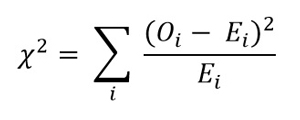
When the R chisq.test function is called, it first calculates a chi-square statistic. The formula for the statistic is shown in Figure 2. It's best explained by example. For the dice example, the observed counts were (12, 8, 15, 5, 16, 4). The expected counts are (10, 10, 10, 10, 10, 10). The calculated chi-square statistic is:
(12 - 10)^2 / 10 + (8 - 10)^2 / 10 + (15 - 10)^2 / 10 +
(5 - 10)^2 / 10 + (16 - 10)^2 / 10 + (4 - 10)^2 / 10

= 4/10 + 4/10 + 25/10 + 25/10 + 36/10 + 36/10

= 130/ 10 = 13.0
 [Click on image for larger view.]
Figure 2. The Chi-Square Statistic
[Click on image for larger view.]
Figure 2. The Chi-Square Statistic
From a developer's point of view, you really don't need to work directly with the chi-square formula because the chisq.test does all the work for you.
Larger values of chi-square indicate the observed and expected counts are farther apart. Chi-square will fail if any expected count is zero. As it turns out, if any expected count is very small, the calculation can be incorrect. R will give you a warning if this happens. One solution to the small expected count problem is to combine categories. For example, in the sex vs. usage problem, if any of the "high" category of usage counts were small (typically less than 5), you could combine the medium and high category counts.
There are many alternatives to the chi-square test. Examples include the g-test and Fisher's exact test. Regardless of which test you use, it's important to realize that all results are probabilistic and only suggest patterns in your data, rather than prove that patterns exist.
About the Author
Dr. James McCaffrey directs the data science and research efforts at Quaetrix, a data analytics company located near Redmond, Washington. Before joining Quaetrix, James was a senior research engineer at Microsoft. James can be reached at [email protected].