The Data Science Lab
DNN Image Classification Using Keras
An example of an image classification problem is to identify a photograph of an animal as a "dog" or "cat" or "monkey." The two most common approaches for image classification are to use a standard deep neural network (DNN) or to use a convolutional neural network (CNN). In this article I'll explain the DNN approach, using the Keras code library.
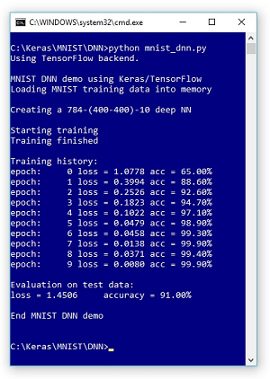
Take a look at Figure 1 to see where this column is headed. The demo program creates an image classification model for a small subset of the MNIST ("modified National Institute of Standards and Technology") image dataset.
The training dataset consists of 1,000 images of handwritten digits. Each image is 28 wide by 28 pixels high (784 pixels) and represents a "0" through a "9."
The demo program creates a standard neural network with 784 input nodes (one for each pixel), two hidden layers, each with 400 processing nodes, and 10 output nodes (one for each possible digit).
The model is trained using 10 epochs (passes through the 1,000 items). The loss (also known as training error) slowly decreases and the prediction accuracy slowly increases, indicating training is working.
After training completed, the demo applied the trained model to a test dataset of 100 items. The model's accuracy is 91.00 percent so 91 of the 100 test images were correctly classified.
 [Click on image for larger view.]
Figure 1. Image Classification Using a DNN with Keras
[Click on image for larger view.]
Figure 1. Image Classification Using a DNN with Keras
This article assumes you have intermediate or better programming skill with a C-family language, but doesn't assume you know much about Keras or neural networks.
The demo is coded using Python, but even if you don't know Python, you should be able to follow along without too much difficulty. The code for the demo program is presented in its entirety in this article. The two data files used are available in the download that accompanies this article.
Understanding the Data
The complete MNIST dataset consists of 60,000 images for training and 10,000 images for testing.
The training set is contained in two files, one that contains all the pixel values and one that contains the associated label values ("0" through "9"). The test images are also contained in two separate files.
Additionally, the four source files are stored in a binary format. When working with deep neural networks, getting the data into a usable form is often the most time-consuming and difficult part of the project.
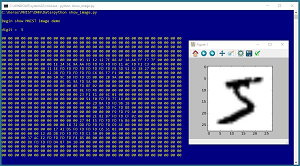
The screenshot in Figure 2 shows the contents of the first training image. The key point is that each image has 784 pixels, and each pixel is a value between 00h (0 decimal) and FFh (255 decimal).
 [Click on image for larger view.]
Figure 2. An MNIST Image
[Click on image for larger view.]
Figure 2. An MNIST Image
Before writing the Keras demo program, I wrote a Python utility program to read the binary source files and write a subset of their contents to text files that can be easily read into memory. File mnist_train_keras_1000.txt looks like:
0 0 0 0 0 1 0 0 0 0 ** 0 .. 170 52 .. 0
0 1 0 0 0 0 0 0 0 0 ** 0 .. 254 66 .. 0
etc.
Getting the raw MNIST binary data into a text file is not trivial. But if you search the Internet you'll find many different ways to read the binary MNIST data and convert it to text.
There are 1,000 lines of data and each represents one image. The first 10 values represent the digit value. The value is one-hot encoded where the position of the 1 bit indicates the digit. Therefore, the two images above represent a "5" and a "1". There is a dummy "**" separator (just for readability) followed by 784 pixel values, each of which is between 0 and 255. File mnist_test_keras_100.txt has 100 images and uses the same format.
In most neural network problems, you want to normalize the predictor values. Instead of directly normalizing the pixel values in the data files, the demo program normalizes the data after it's loaded into memory, as you'll see shortly.
The Demo Program
The complete demo program, with a few minor edits to save space, is presented in Listing 1. All normal error checking has been removed. I indent with two space characters instead of the usual four to save space. Note that the "\" character is used by Python for line continuation.
Listing 1: Complete Demo Program Listing
# mnist_dnn.py
# Keras 2.1.4 TensorFlow 1.4.0
# Anaconda3 4.1.1 (Python 3.5.2)

import numpy as np
import keras as K

import os
os.environ['TF_CPP_MIN_LOG_LEVEL']='2'

def main():
  print("\nMNIST DNN demo using Keras/TensorFlow ")

  print("Loading MNIST training data into memory \n")
  train_file = ".\\Data\\mnist_train_keras_1000.txt"
  train_x = np.loadtxt(train_file, usecols=range(11,795),
    delimiter=" ",  skiprows=0, dtype=np.float32)
  train_y = np.loadtxt(train_file, usecols=range(0,10),
    delimiter=" ", skiprows=0, dtype=np.float32)

  train_x /= 255  # normalize

  print("Creating a 784-(400-400)-10 deep NN \n")
  np.random.seed(1)
  model = K.models.Sequential()
  model.add(K.layers.Dense(units=400, input_dim=784,
    activation='relu'))
  model.add(K.layers.Dense(units=400,
    activation='relu'))
  model.add(K.layers.Dense(units=10,
    activation='softmax'))
  model.compile(loss='categorical_crossentropy',
    optimizer='rmsprop', metrics=['accuracy'])

  print("Starting training ")
  num_epochs = 10
  h = model.fit(train_x, train_y, batch_size=50,
    epochs=num_epochs, verbose=0)
  print("Training finished \n")

  print("Training history: ")
  for i in range(num_epochs):
    if i % 1 == 0:
      los = h.history['loss'][i]
      acc = h.history['acc'][i] * 100
      print("epoch: %5d loss = %0.4f acc = %0.2f%%" \
        % (i, los, acc))

  test_file = ".\\Data\\mnist_test_keras_100.txt"
  test_x = np.loadtxt(test_file, usecols=range(11,795),
    delimiter=" ",  skiprows=0, dtype=np.float32)
  test_y = np.loadtxt(test_file, usecols=range(0,10),
    delimiter=" ", skiprows=0, dtype=np.float32)

  eval = model.evaluate(test_x, test_y, verbose=0)
  print("\nEvaluation on test data: \nloss = %0.4f \
    accuracy = %0.2f%%" % (eval[0], eval[1]*100) )

  print("\nEnd MNIST DNN demo \n")

if __name__ == "__main__":
  main()
All control logic is in a single main function. Because Keras and TensorFlow are relatively new and are under continuous development, it's a good idea to add a comment detailing which versions are being used (2.1.4 and 1.4.0). It's also a good idea to indicate which distribution of Python you're using.
A detailed description of installing Keras is outside the scope of this article, but briefly you first install Anaconda (which contains Python), then you install TensorFlow (which does all the heavy numerical processing) as a Python add-in package, then you install Keras (which provides a Python API) as a second Python add-in.
The demo program begins by importing the NumPy and Keras packages. Notice that you don't explicitly import TensorFlow.
The demo imports the os package just to suppress some warning messages; in a non-demo scenario you'd want to see such messages.
Loading the Data
The demo program loads the training data into memory like so:
train_file = ".\\Data\\mnist_train_keras_1000.txt"
train_x = np.loadtxt(train_file, usecols=range(11,795),
  delimiter=" ",  skiprows=0, dtype=np.float32)
train_y = np.loadtxt(train_file, usecols=range(0,10),
  delimiter=" ", skiprows=0, dtype=np.float32)
train_x /= 255  # normalize
The arguments passed to the loadtxt() function are mostly self-explanatory. But you have to be a bit careful with the range() function because range(x, y) returns a sequence starting from x, inclusive, up to y-1 inclusive.
And notice the demo code skips the dummy "**" separator at position [10] in the data file. The resulting train_x object is a matrix with 1,000 rows and 784 columns, and train_y is a matrix with 1,000 rows and 10 columns.
After loading, all the pixel values are normalized by dividing by 255. The resulting pixel values will now all be in the range [0.0, 1.0]. Notice that the y-values are not normalized because they represent a one-hot encoding.
Creating the Model
The demo program creates a deep neural network with these statements:
np.random.seed(1)
model = K.models.Sequential()
model.add(K.layers.Dense(units=400, input_dim=784,
  activation='relu'))
model.add(K.layers.Dense(units=400,
  activation='relu'))
model.add(K.layers.Dense(units=10, activation='softmax'))
model.compile(loss='categorical_crossentropy',
  optimizer='rmsprop', metrics=['accuracy'])
It's usually a good idea to explicitly set the NumPy global random number seed so that your results will be reproducible.
Each set of 784 normalized input values act as input to the first hidden layer. The outputs of the first hidden layer act as inputs to the second hidden layer. And then the outputs of the second hidden layer are sent to the output layer.
The two hidden layers use ReLU (rectified linear units) activation which, for image classification, often works better than standard tanh activation. The number of hidden nodes, 400, is a free parameter and must be determined by trial and error.
The softmax activation function on the output layer coerces the output node values to sum to 1.0 so they can be interpreted as probabilities of each of the 10 possible digits.
The DNN uses the rmsprop (root mean squared propagation) algorithm for training because rmsprop is usually much faster than the more common sgd (stochastic gradient descent) algorithm for DNN image classification.
Training the Deep Neural Network
The deep neural network classifier is trained with:
print("Starting training ")
num_epochs = 10
h = model.fit(train_x, train_y,
  batch_size=50, epochs=num_epochs, verbose=0)
print("Training finished \n")
In Keras terminology, an epoch is one pass through all training items. In this example, the batch size is set to 50. This means that the training routine will process 50 items at a time and then update the DNN weights. Therefore, because there are 1,000 training items, one epoch will process 20 batches of items. I set the verbose parameter value to 0 to suppress progress messages but in a non-demo scenario you should set verbose to 1 or 2.
The fit() function returns a History object that holds the loss/error and classification accuracy (percentage correct predictions). The demo program displays the History object like so:
for i in range(num_epochs):
  if i % 1 == 0:
    los = h.history['loss'][i]
    acc = h.history['acc'][i] * 100
    print("epoch: %5d loss = %0.4f acc = %0.2f%%" \
      % (i, los, acc))
Here, using modulo 1 means history information will be displayed for every epoch. In situations where you have a much larger History object, you could display every tenth or every hundredth epoch by using modulo 10 or modulo 100.
Evaluating the Trained Model
The demo program evaluates the trained model using these statements:
test_file = ".\\Data\\mnist_test_keras_100.txt"
test_x = np.loadtxt(test_file, usecols=range(11,795),
  delimiter=" ",  skiprows=0, dtype=np.float32)
test_y = np.loadtxt(test_file, usecols=range(0,10),
  delimiter=" ", skiprows=0, dtype=np.float32)
eval = model.evaluate(test_x, test_y, verbose=0)
print("\nEvaluation on test data: \nloss = %0.4f \
  accuracy = %0.2f%%" % (eval[0], eval[1]*100) )
The test input pixel values and the target digit values are loaded into memory in exactly the same way as the training data was loaded because the test data has the same format as the training data. The evaluate() function returns a Python list object where the value at [0] is the total loss (as opposed to average loss) and the value at [1] is the proportion of items that were correctly classified.
Wrapping Up
In a non-demo situation, you'd probably want to save your trained model, so you could load it from a different program. Code to do that would look like:
model.save(".\\mnist_model.h5")

model = K.models.load_model(".\\mnist_model.h5")
And the whole point of creating a model is to make predictions on new, previously unseen data. For example:
pixels_list = [0.55] * 784
pixels_vec = np.array(pixels_list,
  dtype=np.float32)
pixels_mat = pixels_vec.reshape((1,784))
pred_probs = model.predict(pixels_mat)
pred_digit = np.argmax(pred_probs)
print(pred_digit)
This code sets up a dummy image where each pixel is 0.55 (normalized) in a matrix with one row and 784 columns. The pixels are fed to the model using the predict() function. The return value is an array of 10 probabilities, where the largest corresponds to the predicted digit.
Using a standard DNN works well for small images but for large images using a CNN is a better approach. I'll explain how to use a CNN with Keras for large image classification in a future column.
About the Author
Dr. James McCaffrey directs the data science and research efforts at Quaetrix, a data analytics company located near Redmond, Washington. Before joining Quaetrix, James was a senior research engineer at Microsoft. James can be reached at [email protected].