The Data Science Lab

Self-Organizing Maps Using Python

• By James McCaffrey
• 01/15/2019

A self-organizing map (SOM) is a bit hard to describe. Briefly, a SOM is a data structure that allows you to investigate the structure of a set of data. If you have data without class labels, a SOM can indicate how many classes there are in the data. If you have data with class labels, a SOM can be used for dimensionality reduction so the data can be graphed, where the resulting graph indicates how similar different classes are.

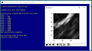
Take a look at a demo program in Figures 1 and 2. The demo begins by creating a 30 x 30 SOM for the well-known Fisher's Iris dataset. The SOM is a data structure in memory. The demo uses the SOM to create what's called a U-Matrix, shown in Figure 1. In a U-Matrix, black cells indicate data items that are similar to each other and white cells indicate borders between groups of similar items. If you squint at the figure you can see that there appears to be three different areas of similar items, suggesting the data has three classes (which it does).

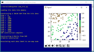
The demo data has labels. There are three labels: 0, 1, 2. In such situations it's possible to use a SOM to visualize the data as shown in Figure 2. This is an example of dimensionality reduction for visualization. The dataset has four dimensions, so it can't be graphed directly.

A SOM can be used to reduce the number of dimensions in a dataset down to two, so the data can be graphed. The image in Figure 2 suggests that the items of class 0 (brown) are most different from items of class 2 (blue), and that items of class 1 (green) are somewhat similar to items of class 0 and class 2.

This article assumes you have intermediate or better programming skill with a C-family language and a basic familiarity with machine learning but doesn't assume you know anything about SOMs. The demo program uses the Anaconda3 version 5.2.0 distribution (Python 3.6.5) but any Python3 version should work.

The demo code is presented in its entirety in this article. The complete source code and the data used are available in the accompanying file download. All normal error checking has been removed to keep the main ideas as clear as possible.

Understanding SOMs
The iris data file has 150 items. The file looks like:

5.1,3.5,1.4,0.2,0
4.9,3.0,1.4,0.2,0
7.0,3.2,4.7,1.4,1
6.3,3.3,6.0,2.5,2

Each line represents an iris flower. The first four values on each line are the flower's sepal length, sepal width, petal length and petal width. Therefore, the data has four dimensions. Because the predictor values all have roughly the same magnitude, it's not necessary to normalize the data, but in most SOM scenarios you'll want to normalize your data. The last item on each line represents the species of the flower: 0 for setosa, 1 for versicolor, 2 for virginica.

The demo SOM is a 30 x 30 matrix where each cell/node holds a vector with four values, such as (5.5, 2.9, 3.8, 1.7). The dimensions of a SOM are arbitrary to a large extent and are mostly a matter of trial and error.

A SOM is created so that each node vector is representative of some of the data items but also so that map nodes that are close to each other geometrically represent data items that are similar. The algorithm used to create the demo SOM, in very high-level pseudo-code is:

create n x n map with random node vector values
loop while s < StepsMax times
  compute what a "close" node means, based on s
  compute a learn rate, based on s
  pick a random data item
  determine the map node closest to data item (BMU)
  for-each node close to the BMU
    adjust node vector values towards data item
end-loop

Creating a SOM is really more of a meta-heuristic than a rigidly prescribed algorithm. Each of the statements in the pseudo-code can be implemented in several ways.

The Demo Program
The structure of demo program, with a few minor edits to save space, is presented in Listing 1. I indent with two spaces rather than the usual four spaces to save space. Note that Python uses the "\" character for line continuation. I used Notepad to edit my program. Most of my colleagues prefer a more sophisticated editor, but I like Notepad.

Listing 1: The Image Classification Demo Program Structure

# som_iris.py
# SOM for Iris dataset
# Anaconda3 5.2.0 (Python 3.6.5)

# ========================================================

import numpy as np
import matplotlib.pyplot as plt

def closest_node(data, t, map, m_rows, m_cols): . .
def euc_dist(v1, v2): . .
def manhattan_dist(r1, c1, r2, c2): . .
def most_common(lst): . .

def main():
  # 0. get started
  np.random.seed(1)
  Dim = 4
  Rows = 30; Cols = 30
  RangeMax = Rows + Cols
  LearnMax = 0.5
  StepsMax = 5000

  # 1. load data into memory
  # 2. construct the SOM
  # 3. construct and display U-Matrix
  # 4. construct and display reduced data

if __name__=="__main__":
  main()

The demo program is named som_iris.py and it starts by importing the NumPy and MatPlotLib packages. There are four helper functions. Function closest_node() returns the row and column indices in the SOM with size m_rows x m_cols that are the coordinates of the map cell whose vector is closest to the data item at data[t]. The cell vector that's closest to a specified data item is called the best matching unit (BMU) in SOM terminology.

Function euc_dist() returns the Euclidean distance between two vectors. For example, if v1 = (2, 1, 4) and v2 = (5, 1, 8) then euc_dist() = sqrt( (5 - 2)^2 + (1 - 1)^2 + (8 - 4)^2 ) = sqrt(25) = 5.0. Function manhattan_dist() returns the Manhattan distance between two cells with coordinates (r1, c1) and (r2, c2). For example, the Manhattan distance between the cells at (2, 5) and (6, 8) is 4 + 3 = 8.

Function most_common() returns the most common value from a list of integer values. For example, if a list held values [0, 2, 2, 1, 0, 1, 1, 2, 1] then most_common() returns 1.

Variables Dim, Rows, Cols hold the dimensionality of the dataset, and the number of rows and columns in the SOM. Variable RangeMax is the maximum Manhattan distance for any two cells in the SOM. Variable LearnMax is the initial learning rate used when constructing the SOM. Variable StepsMax specifies the number of training iterations to perform.

Loading the Data into Memory
The iris data is loaded into memory using these three statements:

  data_file = ".\\Data\\iris_data_012.txt"
  data_x = np.loadtxt(data_file, delimiter=",", usecols=range(0,4),
    dtype=np.float64)
  data_y = np.loadtxt(data_file, delimiter=",", usecols=[4],
    dtype=np.int)

The program assumes that file iris_data_012.txt is located in a subdirectory named Data. In a non-demo scenario you should definitely min-max normalize the data so that features with large magnitudes don't overwhelm features with small values. To keep the demo simple, the demo data is not normalized.

Constructing the SOM
The SOM is created like so:

  print("Constructing a 30x30 SOM from the iris data")
  map = np.random.random_sample(size=(Rows,Cols,Dim))

The call to random_sample() generates a 30 x 30 matrix where each cell is a vector of size 4 with random values between 0.0 and 1.0. The creation of the SOM starts with statements:

  for s in range(StepsMax):
    if s % (StepsMax/10) == 0: print("step = ", str(s))
    pct_left = 1.0 - ((s * 1.0) / StepsMax)
    curr_range = (int)(pct_left * RangeMax)
    curr_rate = pct_left * LearnMax

The pct_left variable computes the percentage of iteration steps remaining. For example if StepsMax is 100 and the current value of s = 25, then pct_left is 0.75 (75 percent). The curr_range variable is the maximum Manhattan distance at step s that defines "close." For example, if s = 25, then the farthest distance two "close" cells can be a cell can be is 60 * 0.75 = 45.

Next, a random data item is selected and the best matching unit map node/cell is determined:

    t = np.random.randint(len(data_x))
    (bmu_row, bmu_col) = closest_node(data_x, t, map, Rows, Cols)

Next, each node/cell of the SOM is examined. If the current node is "close" to the best matching unit node, then the vector in the current node is updated:

    for i in range(Rows):
      for j in range(Cols):
        if manhattan_dist(bmu_row, bmu_col, i, j) < curr_range:
          map[i][j] = map[i][j] + curr_rate *
         (data_x[t] - map[i][j])

The update moves the current node vector closer to the current data item using the curr_rate value which slowly decreases over time.

Constructing the U-Matrix
At this point in the demo, the SOM has been created. Each of the 30 x 30 vectors holds a value that corresponds to one or more data items. The U-Matrix is created from the SOM like so:

  print("Constructing U-Matrix from SOM")
  u_matrix = np.zeros(shape=(Rows,Cols), dtype=np.float64)

Initially, each 30 x 30 cell of the U-Matrix holds a 0.0 value. Next, each cell in the U-Matrix is processed:

  for i in range(Rows):
    for j in range(Cols):
      v = map[i][j]  # a vector 
      sum_dists = 0.0; ct = 0

The value v is the vector in the SOM that corresponds to the current U-Matrix cell. Each adjacent cell in the SOM (above, below, left, right) is processed and the sum of the Euclidean distances is computed:

      if i-1 >= 0:    # above
        sum_dists += euc_dist(v, map[i-1][j]); ct += 1
      if i+1 <= Rows-1:   # below
        sum_dists += euc_dist(v, map[i+1][j]); ct += 1
      if j-1 >= 0:   # left
        sum_dists += euc_dist(v, map[i][j-1]); ct += 1
      if j+1 <= Cols-1:   # right
        sum_dists += euc_dist(v, map[i][j+1]); ct += 1

For example, suppose some cell in the SOM holds (2.0, 1.0, 1.5, 0.7) and the Euclidean distances to the four neighbor cells are 7.0, 12.5, 11.5, 5.0, then the corresponding cell in the U-Matrix holds 36.0 before averaging and then 9.0 after averaging:

      u_matrix[i][j] = sum_dists / ct

A small value in a U-Matrix cell indicates that the corresponding cell in the SOM is very close to its neighbors and therefore the neighboring cells are part of a similar group. The U-Matrix is displayed using the MatPlotLib library:

  plt.imshow(u_matrix, cmap='gray')  # black = close = clusters
  plt.show()

Using a SOM for Dimensionality Reduction Visualization
In situations where your data has class labels, a SOM can be used to reduce dimensionality so the data can be displayed as a two-dimensional graph. First the demo sets up a 30 x 30 matrix where each cell holds an empty list:

  print("Associating each data label to one map node ")
  mapping = np.empty(shape=(Rows,Cols), dtype=object)
  for i in range(Rows):
    for j in range(Cols):
      mapping[i][j] = [] # empty list

Next, each cell is processed and the class label (0, 1 or 2) associated with the data item that is closest to the corresponding cell in the SOM is added to the cell list:

  for t in range(len(data_x)):
    (m_row, m_col) = closest_node(data_x, t, map, Rows, Cols)
    mapping[m_row][m_col].append(data_y[t])

Next, the most common class label is extracted from the list in the current cell and placed into a matrix named label_map:

  label_map = np.zeros(shape=(Rows,Cols), dtype=np.int)
  for i in range(Rows):
    for j in range(Cols):
      label_map[i][j] = most_common(mapping[i][j], 3)

At this point the 30 x 30 matrix label_map holds a -1 if no data items are associated with the cell, or a value 0, 1 or 2 indicating the most common class label associated with the cell. The demo concludes by displaying this reduced dimensionality matrix:

  plt.imshow(label_map, cmap=plt.cm.get_cmap('terrain_r', 4))
  plt.colorbar()
  plt.show()
if __name__=="__main__":
  main()

The 4 argument passed to get_cmap() takes into account that you want four colors: one for each of the three class labels plus one color to indicate no associated class label.

Wrapping Up
There are dozens of variations of the basic self-organizing map structure used in the demo program. Instead of using a n-by-m rectangular grid, you can use a layout where each cell in the SOM is a hexagon. You can use a toroidal geometry where edges of the SOM connect. You can use three dimensions instead of two. There are many ways to define a close neighborhood for nodes. And so on.

At least among my colleagues, SOMs aren't used very often. I suspect there are several reasons for this but perhaps the main reason is that SOMs have so many variations it's rather confusing to select one particular design. Additionally, based on my experience, in order for a SOM to give useful insights into a dataset, a custom SOM is needed (as opposed to using an off-the-shelf SOM from a machine learning library.) All that said however, for certain problem scenarios, SOMs can provide useful insights into the structure of a dataset.

• Get Code Download