The Data Science Lab
How to Do Neural Network Glorot Initialization Using Python
Microsoft Research data scientist Dr. James McCaffrey explains what neural network Glorot initialization is and why it's the default technique for weight initialization.
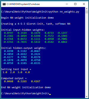
In this article I explain what neural network Glorot initialization is and why it's the default technique for weight initialization. The best way to see where this article is headed is to take a look at the screenshot of a demo program in Figure 1.
The demo program creates a single hidden layer neural network that has 4 input nodes, 5 hidden processing nodes and 3 output nodes. The network weights are initialized using the Glorot uniform technique.
 [Click on image for larger view.]
Figure 1.Neural Network Glorot Initialization Demo Program
[Click on image for larger view.]
Figure 1.Neural Network Glorot Initialization Demo Program
The demo displays the randomly initialized values of the 20 input-to-hidden weights and the 15 hidden-to-output weights. All the weight values are between -1.0 and +1.0. The demo concludes by sending test input of (1.0, 2.0, 3.0, 4.0) to the network. The computed output values are (0.0468, 0.5265, 0.4267). The output values sum to 1.0 because the neural network uses softmax output activation.
This article assumes you have a basic familiarity with Python or a C-family language such as C# or JavaScript, but doesn't assume you know anything about Glorot initialization. The demo program is too long to completely present in this article, but the two source code files used are available in the accompanying file download.
I wrote the demo using the 3.6.5 version of Python and the 1.14.3 version of NumPy but any relatively recent versions will work fine. It's possible to install Python and NumPy separately, however, if you're new to Python and NumPy I recommend installing the Anaconda distribution of Python which simplifies installation and gives you many additional useful packages.
Understanding Glorot Initialization
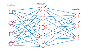
The diagram in Figure 2 represents a 4-5-3 neural network. The blue lines connecting input nodes to the hidden nodes and the hidden nodes to the output nodes represent the network's weights. These are just constants with values like 0.1234 and -1.009. The short purple arrows pointing into each hidden node and each output node represent the network's biases which are also just numeric constants.
 [Click on image for larger view.]
Figure 2.Neural Network Weights and Biases
[Click on image for larger view.]
Figure 2.Neural Network Weights and Biases
For a 4-5-3 network there are (4 * 5) + (5 * 3) = 35 weights and 5 + 3 = 8 biases. In general, if there are ni input nodes, nh hidden nodes and no output nodes there are (ni * nh) + (nh * no) weights and nh + no biases. The values of the output nodes are determined by the values of the input nodes and the values of the weights and biases. Training a network is the process of finding values for the weights and biases so that the network makes accurate predictions on training data that has known input values and known correct output (also called target) values.
Before training a network, you must initialize the values of the weights. In most situations the biases are initialized to 0.0 and so initialization isn't an issue for biases. As it turns out, neural networks are surprisingly sensitive to the initial weight values and so weight initialization is important.
In the early days of neural networks the most common technique for weight initialization was to set the values to small uniform random values between two arbitrary limits, for example random values between -0.01 and +0.01. This technique works reasonably well but has two drawbacks. First, there's no good way to determine the initialization limit values. Second, because different data scientists use different initialization limit values, and rarely document what those values are, replicating other people's results is often difficult or impossible.
Code that uses the uniform random with fixed limits initialization approach could look like:
def init_weights(self):
  lo = -0.01; hi = +0.01
  for i in range(self.ni):  # input-hidden wts
    for j in range(self.nh):
      x = np.float32(self.rnd.uniform(lo, hi))
      self.ih_weights[i,j] = x
  # similarly for hidden-output weights
The Glorot weight initialization algorithm is named after the lead author of a technical paper that described the technique. There are actually two versions of Glorot initialization: Glorot uniform and Glorot normal. The algorithm is best explained using code. Here's Glorot uniform for the input-hidden weights:
def init_weights(self):  # Glorot uniform
  nin = self.ni; nout = self.nh
  sd = np.sqrt(6.0 / (nin + nout))
  for i in range(self.ni):
    for j in range(self.nh):
      x = np.float32(self.rnd.uniform(-sd, sd))
      self.ih_weights[i,j] = x
. . .
Here ni and nh are the number of input and hidden nodes. The nin and nout stand for "number in" and number out". These are sometimes called the "fan-in" and the "fan-out". In short, instead of using fixed limits like -0.01 and +0.01, Glorot uniform initialization uses limits that are based on the number of nodes in the network: sqrt( 6 / (nin + nout)).
For the 4-5-3 demo neural network input-hidden weights, nin = 4 and nout = 5, therefore sd = sqrt(6/9) = 0.82 and so all input-hidden weights will be random values between -0.82 and +0.82.
Initialization for the hidden-output weights follows the same pattern:
  nin = self.nh; nout = self.no
  sd = np.sqrt(6.0 / (nin + nout))
  for j in range(self.nh):
    for k in range(self.no):
      x = np.float32(self.rnd.uniform(-sd, sd))
      self.ho_weights[j,k] = x
The Glorot initialization technique not only works better (in most cases) than uniform random initialization but Glorot also eliminates the need for you to guess good values of fixed limits. Nice!
The Glorot normal initialization technique is almost the same as Glorot uniform. The limit value is sqrt( 2 / (nin + nout)) and the random values are pulled from the normal (also called Gaussian) distribution instead of the uniform distribution:
def init_weights(self):  # Glorot normal
  nin = self.ni; nout = self.nh
  sd = np.sqrt(2.0 / (nin + nout))
  for i in range(self.ni):
    for j in range(self.nh):
      x = np.float32(self.rnd.normal(0.0, sd))
      self.ih_weights[i,j] = x
. . .
Glorot uniform and Glorot normal seem to work about equally well, especially for neural networks with a single hidden layer. Glorot initialization is sometimes called Xavier initialization, after the Glorot's first name. There is a closely related initialization algorithm called He normal initialization, where the limit value is sqrt( 2 / nin).
Overall Program Structure
The overall program structure, with a few minor edits to save space, is presented in Listing 1. To edit the demo program I used the basic Notepad program. Most of my colleagues prefer using one of the many nice Python editors that are available. I indent with two spaces rather than the usual four.
I commented the name of the program and indicated the Python version used. I placed utility functions, such as show_vec() and hypertan() in a file named my_utilities.py and placed that file in a directory named Utilities.
Listing 1: Overall Program Structure
# nn_weights.py
# Python 3.6.5

import sys
sys.path.insert(0, "..\\Utilities")
import my_utilities as U
import numpy as np

# ------------------------------------

class NeuralNetwork: . . .

# ------------------------------------

def main():
  print("Begin NN weight initialization demo ")

  # 1. create network
  print("Creating 4-5-3 Glorot, tanh, softmax NN")
  seed = 0
  nn = NeuralNet(4, 5, 3, seed)

  # 2. display initial weights
  print("Initial input-hidden weights:")
  print("\033[0m" + "\033[92m", end="") # green
  for i in range(nn.ni):
    for j in range(nn.nh):
      wt = nn.ih_weights[i,j]
      print("%8.4f" % wt + " " , end="")
    print("")
  print("\033[0m", end="") # reset

  print("Initial hidden-output weights:")
  print("\033[0m" + "\033[96m", end="") # cyan
  for j in range(nn.nh):
    for k in range(nn.no):
      wt = nn.ho_weights[j,k]
      print("%8.4f" % wt + " " , end="")
    print("")
  print("\033[0m", end="") # reset

  # 3. test NN input-output
  inpt = np.array([1.0, 2.0, 3.0, 4.0],
    dtype=np.float32)
  print("Setting test input = ")
  U.show_vec(inpt, 4, 1, len(inpt))
  oupt = nn.eval(inpt)
  print("Computed output = ")
  U.show_vec(oupt, 8, 4, len(oupt))

  print("End NN weight initialization demo ")

if __name__ == "__main__":
  main()
The demo program consists mostly of a program-defined NeuralNetwork class. I created a main function to hold all program control logic. The Glorot initiation is invoked when the neural network is created. The constructor method has code:
class NeuralNet:
  def __init__(self, num_input, num_hidden, \
    num_output, seed):
    self.ni = num_input
    self.nh = num_hidden
    self.no = num_output
    # set up storage for nodes, weights, etc.
    self.rnd = np.random.RandomState(seed)
    self.init_weights()
The class has a RandomState object to generate random numbers for the initialization code. The random object is initialized with a seed value so that results are reproducible.
Wrapping Up
The creation of code libraries such as TensorFlow and PyTorch for deep neural networks has greatly simplified the process of implementing sophisticated neural prediction models such as convolutional neural networks and LSTM networks. However, these neural libraries are very complex and require significant time and effort to learn. For many problems, a simple neural network with a single hidden layer is effective, and implementing such a network using raw Python is practical and efficient.
About the Author
Dr. James McCaffrey directs the data science and research efforts at Quaetrix, a data analytics company located near Redmond, Washington. Before joining Quaetrix, James was a senior research engineer at Microsoft. James can be reached at [email protected].