The Data Science Lab
How to Train a Machine Learning Radial Basis Function Network Using C#
A radial basis function network (RBF network) is a software system that's similar to a single hidden layer neural network, explains Dr. James McCaffrey of Microsoft Research, who uses a full C# code sample and screenshots to show how to train an RBF network classifier.
A radial basis function network (RBF network) is a software system that is similar to a single hidden layer neural network. In this article I explain how to train an RBF network classifier. I use the C# language but you shouldn't have any trouble refactoring the demo code to another programming language if you wish.
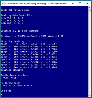
A good way to see where this article is headed is to take a look at the demo program shown in the screenshot in Figure 1 and the graph in Figure 2. The demo begins by setting up a 2-15-3 RBF network. There are two input nodes, 15 hidden nodes, and three output nodes. You can imagine that the RBF network corresponds to a problem where the goal is to predict a person's political leaning (conservative, moderate, liberal) based on their age and annual income.
The number of input and number of output nodes in an RBF network are determined by the problem data, but the number of hidden nodes (15 in the demo) is a hyperparameter that must be determined by trial and error.
There are 28 training items. The data is artificial and was crafted so that simple linear classification techniques, such as multi-class logistic regression and linear SVM, would fail.
The demo program sets values for three training hyperparameters: a learning rate (0.0050), maximum number of iterations (1000), and a single sigma value for the network (0.10). During training, the classification mean squared error slowly decreases from an initial 0.6654 to 0.3272, indicating that training is working.
After training completes, the demo makes a prediction for a new, previously unseen data item with normalized predictor values (0.15, 0.25). The output of the trained RBF model is (0.1354, 0.3190, 0.5455). If the three classes to predict are conservative = (1, 0, 0), moderate = (0, 1, 0), and liberal = (0, 0, 1) then the predicted class would be liberal.
 [Click on image for larger view.] Figure 1: RBF Network Training Demo
This article assumes you have intermediate or better skill with C# and a solid understanding of RBF network architecture and the RBF network input-output mechanism but doesn’t assume you know anything about training RBF networks. You can find an article explaining RBF network architecture and IO in the list of Visual Studio Magazine Data Science Lab articles.
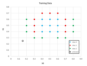 [Click on image for larger view.] Figure 2: Training Data
The code for demo program is a bit too long to present in its entirety in this article but the complete source code is available in the associated file download.
Understanding RBF Network Training
The diagram in Figure 3 shows the architecture of a 3-4-2 RBF network. There are three input nodes, or equivalently, an input vector with three values. There are four hidden nodes. Each hidden node has a centroid which is a vector with the same number of values as the input. RBF centroids are usually given the symbol Greek lowercase mu (μ) or English lowercase u.
Each hidden node has a width (sometimes called a standard deviation) which is a single numeric value. RBF widths are usually given the symbol Greek lowercase sigma (σ) or English lowercase s. And each hidden node has a node value which is a single numeric value. There is no standard symbol for a hidden node value.
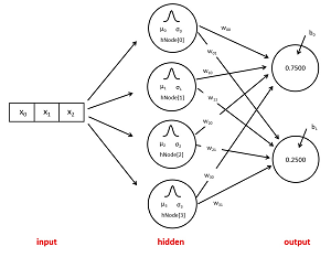 [Click on image for larger view.] Figure 3: Example 3-4-2 RBF Network Architecture
The 3-4-2 RBF network in Figure 3 has two output nodes. For an RBF classifier network, the output node values will be normalized so that they sum to 1.0 (for example 0.75 and 0.25) and can be loosely interpreted as probabilities. Each output node has an associated bias value. Bias values are usually given the symbol Greek lowercase beta ( β) or English lowercase b.
An RBF network has a weight value associated with each hidden-to-output node connection. A 3-4-2 network has 4 * 2 = 8 weights. The 2-15-3 RBF demo network has 15 * 3 = 45 weights.
The computed output of an RBF network depends on the input values, and the values of the centroids, the widths, the weights and the biases. Training an RBF network is the process of finding the values of the centroids, widths, weights and biases.
Setting the Values of the Hidden Node Centroids and Widths
There are several approaches for specifying the values of the centroids. The approach I recommend is to select random training items and use them as the values of the centroids. For example, the demo 2-15-3 RBF network requires 15 centroids, where each centroid has two values. The demo training data has 28 items. To supply values for the centroids, the demo Train() method selects 15 of the 28 training items and then copies the values of the 15 selected training items to the 15 RBF centroids.
Suppose you have a 2-4-3 RBF network and you have 8 training data items:
[0] (0.1, 0.19) -> (1, 0, 0)
[1] (0.2, 0.18) -> (0, 1, 0)
[2] (0.3, 0.17) -> (0, 0, 1)
[3] (0.4, 0.16) -> (0, 1, 0)
[4] (0.5, 0.15) -> (1, 0, 0)
[5] (0.6, 0.14) -> (0, 0, 1)
[6] (0.7, 0.13) -> (0, 1, 0)
[7] (0.8, 0.12) -> (1, 0, 0)
To select four random items, first you'd set up an ordered array of eight indices:
(0, 1, 2, 3, 4, 5, 6, 7)
Then you shuffle the indices using the Fisher-Yates mini-algorithm giving something like:
(6, 7, 0, 5, 1, 3, 4, 2)
Then you'd use the first four shuffled indices to pluck off four training items:
[6] (0.7, 0.13)
[7] (0.8, 0.12)
[0] (0.1, 0.19)
[5] (0.6, 0.14)
And then you'd copy these values into the four centroids. Notice that this approach for setting the values of the centroids isn't at all like machine learning training in the usual sense where you iteratively find better values.
There are several approaches for setting the values of the hidden node widths. The approach I recommend is to use a single value for all widths. For example, the demo program sets all 15 widths to 0.10. This value was found by trial and error.
RBF networks are highly sensitive to the value(s) of the hidden node widths and finding good value(s) for the widths is often the biggest challenge when training an RBF network. Researchers have tried many complex algorithms for setting the values of RBF widths but there is no solid evidence that any of these complex technique work better than using a single common width value.
Training the Values of the Weights and Biases
The most common technique for training the values of RBF network weights and biases (which can be thought of as special weights) is to use one of several forms of stochastic gradient descent.
 [Click on image for larger view.] Figure 4: The RBF Weight Update Equation
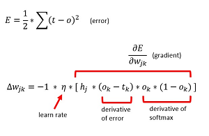
The underlying error function and the weight update equation, in math form, are shown in Figure 4. In words, the error is one half the sum of the squared target values minus output values. For example, suppose there are just three training items:
targets     computed output
---------------------------
(0, 1, 0)   (0.1, 0.7, 0.3)
(1, 0, 0)   (0.6, 0.2, 0.2)
(0, 0, 1)   (0.4, 0.1, 0.5)
The error of the first item is (0 – 0.1)^2 + (1 – 0.7)^2 + (0 – 0.3)^2 = 0.01 + 0.09 + 0.09 = 0.19. Similarly, the error of the second item is 0.24 and the error of the third item is 0.42. The total error is 1/2 * (0.19 + 0.24 + 0.42). The one-half term is included only so that the derivative of the error is simpler. In practice, you usually just compute mean squared error, which for the three example items, would be (0.19 + 0.24 + 0.42) / 3. Notice that all three training items are correctly predicted because the largest computed output probability corresponds to the 1 value in the target.
In the weight update equation, delta wjk is the amount to add to the weight connecting hidden node j with output node k. Greek letter eta (η) is the learning rate which moderates the weight delta. The symbol hj is the value of hidden node j. The tk term is the target value for output node k and the ok term is the computed output value for output node k.
The mysterious-looking -1 term in the weight update equation is included so only the weight delta is added to the current weight value, rather than subtracted. This is the common form used in standard neural network training, so I use that convention for RBF networks too.
The Demo Program
To create the demo program, I launched Visual Studio 2019. I used the Community (free) edition but any relatively recent version of Visual Studio will work fine. From the main Visual Studio start window I selected the "Create a new project" option. Next, I selected C# from the Language dropdown control and Console from the Project Type dropdown, and then picked the "Console App (.NET Core)" item.
The code presented in this article will run as a .NET Core console application or as a .NET Framework application. Many of the newer Microsoft technologies, such as the ML.NET code library, specifically target the .NET Core framework so it makes sense to develop most new C# machine learning code in that environment.
I entered "RadialNetMulti" as the Project Name, specified C:\VSM on my local machine as the Location (you can use any convenient directory), and checked the "Place solution and project in the same directory" box.
After the template code loaded into Visual Studio, at the top of the editor window I removed all using statements to unneeded namespaces, leaving just the reference to the top-level System namespace. The demo needs no other assemblies and uses no external code libraries.
In the Solution Explorer window, I renamed file Program.cs to the more descriptive RadialNetMultiProgram.cs and then in the editor window I renamed class Program to class RadialNetMultiProgram to match the file name. The structure of the demo program, with a few minor edits to save space, is shown in Listing 1.
Listing 1. RBF Network Training Demo Program
using System;
namespace RadialNetMulti
{
  class RadialNetMultiProgram
  {
    static void Main(string[] args)
    {
      Console.WriteLine("Begin RBF network demo ");

      double[][] trainX = new double[28][];
      trainX[0] = new double[] { 0.4, 0.6 };   // 0
      trainX[1] = new double[] { 0.5, 0.6 };
      . . .
      trainX[9] = new double[] { 0.4, 0.7 };   // 1
      trainX[10] = new double[] { 0.5, 0.7 };
      . . .
      trainX[18] = new double[] { 0.2, 0.6 };  // 2
      . . .
      trainX[27] = new double[] { 0.6, 0.3 };

      int[][] trainY = new int[28][];
      trainY[0] = new int[] { 1, 0, 0 };   // 0
      trainY[1] = new int[] { 1, 0, 0 };
      . . .
      trainY[9] = new int[] { 0, 1, 0 };   // 1
      trainY[10] = new int[] { 0, 1, 0 };
      . . .
      trainY[18] = new int[] { 0, 0, 1 };  // 2
      . . .
      trainY[27] = new int[] { 0, 0, 1 };

      Console.WriteLine("Creating 2-15-3 RBF ");
      RadialNet rn = new RadialNet(2, 15, 3, 0);

      double lr = 0.005;
      int maxEpoch = 1000;
      double sigma = 0.1;
      Console.WriteLine("Setting lr = " +
        lr.ToString("F4") +
        " maxEpoch = " + maxEpoch +
        " sigma = " + sigma.ToString("F2"));

      Console.WriteLine("Starting training");
      rn.Train(trainX, trainY, lr, sigma, maxEpoch);
      Console.WriteLine("Training complete");

      double[] unk = new double[] { 0.15, 0.25 };
      Console.WriteLine("Predicting class for: ");
      ShowVector(unk, 2);

      double[] p = rn.ComputeOutputs(unk);
      Console.WriteLine("Predicted probs: ");
      ShowVector(p, 4);

      Console.WriteLine("End demo ");
      Console.ReadLine();
    } // Main

    public static void ShowVector(double[] v,
      int dec) { . . }

    public static void ShowMatrix(double[][] m,
      int dec) { . . }

  } // Program class

  class RadialNet
  {
    . . .
  }

} // ns
All of the program control logic is contained in the Main() method. Helper functions ShowVector() and ShowMatrix() display a numeric vector or array-of-arrays style matrix using a specified number of digits after the decimal point.
The RBF network definition is contained in a class named RadialNet. All normal error checking has been removed to keep the main ideas as clear as possible.
The demo begins by setting up 28 hard-coded training items:
double[][] trainX = new double[28][];
trainX[0] = new double[] { 0.4, 0.6 };
trainX[1] = new double[] { 0.5, 0.6 };
. . .
int[][] trainY = new int[28][];
trainY[0] = new int[] { 1, 0, 0 };
trainY[1] = new int[] { 1, 0, 0 };
. . .
In a non-demo scenario, you'd likely store training data in a text file like:
0.4, 0.6, 1, 0, 0
0.5, 0.6, 1, 0, 0
. . .
0.6, 0.3, 0, 0, 1
And then load data into memory using program-defined overloaded helper functions along the lines of:
string fn = ".\\trainData.txt";
double[][] trainX = LoadMatrix(fn, new int[] { 0, 1 }, ",");
int[][] trainY = LoadMatrix(fn, new int[] { 2, 3, 4 }, ",");
Next, the demo creates a 2-15-3 RBF network:
Console.WriteLine("Creating 2-15-3 RBF ");
RadialNet rn = new RadialNet(2, 15, 3, 0);
The 0 argument passed to the constructor is a seed value for a Random object in the network. The Random object is used to select random training items for the centroids, to initialize weights to small random values, and to shuffle training items so that they are processed in a different random order on each pass through the data.
Next, the demo prepares and then preforms training:
double lr = 0.005;
int maxEpoch = 1000;
double sigma = 0.1;
rn.Train(trainX, trainY, lr, sigma, maxEpoch);
The learning rate, maximum number of epochs (an epoch is one pass through all training items), and sigma (a common width value for all hidden nodes) are all hyperparameters that must be determined by trial and error.
In a non-demo scenario, after training completes you'd likely want to save the values of the centroids, width, weights and biases to a text file.
The demo program concludes by using the trained RBF network model to make a prediction for a new, previously unseen item:
double[] unk = new double[] { 0.15, 0.25 };
double[] p = rn.ComputeOutputs(unk);
Console.WriteLine("Predicted probs: ");
ShowVector(p, 4);
In a non-demo scenario you might want to consider explicitly displaying the predicted class along the lines of:
string[] labels =
  new string[] { "conservative" , "moderate", "liberal");
int idx = ArgMax(p);  // index of largest prob
string predicted = labels[idx];
Console.WriteLine(predicted);
Implementing RBF Network Training
The demo program implements RBF training in a method named Train(). The method definition begins with:
public void Train(double[][] trainX, int[][] trainY,
  double lr, double sigma, int maxEpoch)
{
  // 1. random centroids
  int[] indices = new int[trainX.Length];
  for (int i = 0; i < indices.Length; ++i)
    indices[i] = i;
  Shuffle(indices, this.rnd);
. . .
This code sets up the indices of the training items and then scrambles them using helper method Shuffle(). The Shuffle() method uses the class Random object, passed in as a parameter. After shuffling the indices, the indices are used to select training items:
for (int j = 0; j <this.nh; ++j)
{
  int idx = indices[j];
  for (int i = 0; i <this.ni; ++i)
    this.centroids[j][i] = trainX[idx][i];
}
The indexing is a bit tricky. The demo indexes input values using i, hidden nodes using j, and output nodes using k. Next, the common value of the widths is set:
// 2. width
for (int j = 0; j < this.nh; ++j)
  this.widths[j] = sigma;
As explained previously, there are many complex techniques that can be used to assign values to the widths associated with each hidden node but the demo uses one common value, passed in as a parameter, for all widths.
After the centroids and widths have been set, the next step is to use stochastic gradient descent to assign values for the weights and biases. First, the values of the weights are initialized to small random values between -0.01 and +0.01 like so:
// 3a.init weights ad hoc technique
double hi = 0.01; double lo = -hi;
for (int j = 0; j < this.nh; ++j)
  for (int k = 0; k < this.no; ++k)
    this.weights[j][k] =
      (hi - lo) * this.rnd.NextDouble() + lo;
The upper and lower limits of +0.01 and -0.01 are hard-coded. Unlike deep neural networks, which are very sensitive to initial weight values, RBF networks tend to be relatively insensitive to initial weight values. The demo leaves the bias values initialized to 0.0 which is a common approach used when training standard neural networks.
After weight initialization, the Train() method iterates maxEpoch times. On each epoch, the indices of the training items are shuffled so that they are processed in a different random order:
// 3b. train weights using online SGD
for (int epoch = 0; epoch < maxEpoch; ++epoch)
{
  Shuffle(indices, this.rnd);  // process in random order
  foreach (int idx in indices) {
    this.ComputeOutputs(trainX[idx]);
    for (int j = 0; j < this.nh; ++j) {
      for (int k = 0; k < this.no; ++k) {
        double delta = -1 * lr *
          (this.oNodes[k] - trainY[idx][k]) *
          this.hNodes[j] * (this.oNodes[k] *
          (1 - this.oNodes[k]));
        this.weights[j][k] += delta;
      }
      // update biases here
    }
  }
. . .
This version of stochastic gradient descent is called online training. All weights are updated after reading one data item. An alternative is to use batch training where all training items are processed and then gradients are accumulated and averaged.
Updating the biases follows the same pattern as updating the weights:
for (int k = 0; k < this.no; ++k) {
  double delta = -1 * lr *
   (this.oNodes[k] - trainY[idx][k]) *
   1 * (this.oNodes[k] * (1 - this.oNodes[k]));
  this.biases[k] += delta;
}
A bias can be thought of as a weight with a constant associated input of 1 so instead of using a hidden node value, h[j], updating a bias uses a constant 1.
The demo program displays progress metrics 10 times during training. Because the value of maxEpoch is set to 1000, metrics are displayed every 100 epochs:
if (epoch % (maxEpoch / 10) == 0) {
  double err = Error(trainX, trainY);
  double acc = Accuracy(trainX, trainY);
  Console.Write("epoch = " + epoch.ToString());
  Console.Write("  error = " + err.ToString("F4"));
  Console.Write("  acc = " + acc.ToString("F4"));
  Console.WriteLine("");

  // display weights here
}
During training, it's important to monitor error to see if training is working. It's also a good idea to display classification accuracy, even though accuracy is a much cruder measure than error. Additionally, I recommend displaying the values of the hidden-to-output weights during training because RBF networks are sometimes subject to severe overfitting where the weight values explode in magnitude.
Wrapping Up
The demo program has inputs with two numeric values, such as (0.45, 0.75). When using RBF networks, it's important to normalize numeric predictor values so that large values (such as an income of $75,000.00) don't overwhelm small values (such as an age of 28).
If you have predictors that are categorical values, such as a job type of "management" or "sales" or "technical," you can one-hot encode them like management = (1, 0, 0), sales = (0, 1, 0), technical = (0, 0, 1). For binary predictor values you can either use one-hot encoding, for example male = (1, 0) and female = (0, 1) or you can use minus-one plus-one encoding, for example male = -1 and female = +1.
In my opinion, there is no solid research evidence to indicate that RBF networks are better than, worse than, or about the same as standard single hidden layer neural networks. One possible use of RBF networks is as part of an ensemble approach. For example, you can create and train a standard neural network model and an RBF network model, and then combine the predictions made by each system for a consensus prediction.