The Data Science Lab
Binary Classification Using a scikit Decision Tree
Dr. James McCaffrey of Microsoft Research says decision trees are useful for relatively small datasets and when the trained model must be easily interpretable, but often don't work well with large data sets and can be susceptible to model overfitting.
A decision tree is a machine learning technique that can be used for binary classification or multi-class classification. A binary classification problem is one where the goal is to predict the value of a variable where there are only two possibilities. For example, you might want to predict the sex of a person (male or female) based on their age, state where they live, income and political leaning. There are many other techniques for binary classification, but using a decision tree is very common and the technique is considered a fundamental machine learning skill for data scientists.
There are several tools and code libraries that you can use to perform binary classification using a decision tree. The scikit-learn library (also called scikit or sklearn) is based on the Python language and is one of the most popular machine learning libraries.
A good way to see where this article is headed is to take a look at the screenshot in Figure 1. The demo program loads a 200-item set training data and a 40-item set of test data into memory. Next, the demo creates and trains a decision tree model using the DecisionTreeClassifier class from the scikit library.
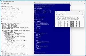 [Click on image for larger view.] Figure 1: Binary Classification Using a scikit Decision Tree
After training, the model is applied to the training data and the test data. The model scores 81.00 percent accuracy (162 out of 200 correct) on the training data, and 77.50 percent accuracy (31 out of 40 correct) on the test data. The demo concludes by displaying the model in pseudo-code format.
This article assumes you have intermediate or better skill with a C-family programming language, but doesn't assume you know much about decision trees or the scikit library. The complete source code for the demo program is presented in this article and the accompanying file download. The source code is also available online.
Installing the scikit Library
There are several ways to install the scikit library. I recommend installing the Anaconda Python package. Anaconda contains a core Python engine plus over 500 libraries that are (mostly) compatible with each other. I used Anaconda3-2020.02 which contains Python 3.7.6 and the scikit 0.22.1 version. The demo code runs on Windows 10 or 11.
Briefly, Anaconda is installed using a Windows self-extracting executable file. The setup process is mostly straightforward and takes about 15 minutes. You can find step-by-step instructions.
There are more up-to-date versions of Anaconda / Python / scikit library available. But because the Python ecosystem has hundreds of libraries, if you install the most recent versions of these libraries, you run a greater risk of library incompatibilities -- a big headache when working with Python.
The Data
The data is artificial and can be found here. There are 200 training items and 40 test items. The structure of data looks like:
1   0.24   1   0   0   0.2950   0   0   1
0   0.39   0   0   1   0.5120   0   1   0
1   0.63   0   1   0   0.7580   1   0   0
0   0.36   1   0   0   0.4450   0   1   0
1   0.27   0   1   0   0.2860   0   0   1
. . .
The tab-delimited fields are sex (0 = male, 1 = female), age (divided by 100), state (Michigan = 100, Nebraska = 010, Oklahoma = 001), income (divided by $100,000) and political leaning (conservative = 100, moderate = 010, liberal = 001). For binary tree classification, the variable to predict should be encoded as 0 or 1. Although it's not technically necessary, I prefer to normalize all predictor values to the same range, typically 0.0 to 1.0 or -1.0 to +1.0. The categorical predictors should be one-hot encoded. For example, if there were five states instead of just three, the states would be encoded as 10000, 01000, 00100, 00010, 00001.
For ordinal predictors that have an implied order, it is possible to use ordinal encoding. For example, a predictor variable such as height with possible values "short," "medium" and "tall" could be encoded as short = 0, medium = 1, height = 2.
Understanding How a Decision Tree Works
The result of training a decision tree classifier is a set of if-then rules. The demo program rules look like:
if ( income <= 0.3400 ) {
   if ( pol2 <= 0.5 ) {
     if ( age <= 0.235 ) {
       if ( income <= 0.2815 ) {
         return 1.0
. . .
For example, a person who has an income of 0.2800 ($28,000) and who is either a conservative or a liberal (i.e., not a moderate), and whose age is 22, is predicted to be class 1 = female. Because the politics type is encoded as conservative = 100, moderate = 010, liberal = 001, the condition pol2 <= 0.5 means the middle encoding value is 0, which means conservative or liberal.
Starting with all 200 training items, the decision tree algorithm scans the data and finds the one value of the one predictor variable that splits the data into two sets in such a way that the most information is obtained. Loosely speaking, you can imagine that for predicting sex, the training algorithm finds a predictor variable (income) and a value (0.3400) so that most male data items have incomes that less than or equal to 0.3400 and most female data items have incomes that are greater than the 0.3400 value.
After the first split, the decision tree algorithm examines each of the two subsets of data and finds a predictor variable and a value that gives the most information. The process continues until a program-specified maximum tree depth is reached.
There are several algorithms to split data. The most common technique is called Gini impurity. The second most common splitting technique is called Shannon information gain.
If a large tree depth value is used, it's possible to generate a very large tree that achieves 100 percent classification accuracy. But such a tree would overfit the training data and give poor accuracy on new, previously unseen data items.
The Demo Program
The complete demo program is presented in Listing 1. Notepad is my preferred code editor but most of my colleagues prefer one of the many excellent code editors that are available. I indent my Python program using two spaces rather than the more common four spaces.
The program imports the NumPy library which contains numeric array functionality. The DecisionTree module has the key code for creating a binary or multi-class decision tree. Notice the name of the root scikit module is sklearn rather than scikit.
The precision_score module contains code to compute precision -- a special type of accuracy for binary classification. The pickle library has code to save a trained model. (The word pickle means to preserve food for later use, as in pickled cucumbers.)
Listing 1: Complete Demo Program
# people_gender_tree.py

# predict gender (0 = male, 1 = female)
# from age, state, income, politics-type

# data:
#  0   0.39   0   0   1   0.5120   0   1   0
#  1   0.27   0   1   0   0.2860   1   0   0
# . . .

# Anaconda3-2020.02  Python 3.7.6
# Windows 10/11  scikit 0.22.1

import numpy as np
from sklearn import tree

# ---------------------------------------------------------

def tree_to_pseudo(tree, feature_names):
  left = tree.tree_.children_left
  right = tree.tree_.children_right
  threshold = tree.tree_.threshold
  features = [feature_names[i] for i in tree.tree_.feature]
  value = tree.tree_.value

  def recurse(left, right, threshold, features, node, depth=0):
    indent = "  " * depth
    if (threshold[node] != -2):
      print(indent,"if ( " + features[node] + " <= " + \
        str(threshold[node]) + " ) {")
      if left[node] != -1:
        recurse(left, right, threshold, features, \
          left[node], depth+1)
        print(indent,"} else {")
        if right[node] != -1:
          recurse(left, right, threshold, features, \
            right[node], depth+1)
        print(indent,"}")
    else:
      idx = np.argmax(value[node])
      # print( indent,"return " + str(value[node]))
      print( indent,"return " + str(tree.classes_[idx]))

  recurse(left, right, threshold, features, 0)

# ---------------------------------------------------------

def main():
  # 0. get ready
  print("\nBegin scikit decision tree example ")
  print("Predict sex from age, state, income, politics ")
  np.random.seed(0)

  # 1. load data
  print("\nLoading data into memory ")
  train_file = ".\\Data\\people_train.txt"
  train_xy = np.loadtxt(train_file, usecols=range(0,9),
    delimiter="\t", comments="#",  dtype=np.float32)
  train_x = train_xy[:,1:9]
  train_y = train_xy[:,0]

  test_file = ".\\Data\\people_test.txt"
  test_xy = np.loadtxt(test_file, usecols=range(0,9),
    delimiter="\t", comments="#",  dtype=np.float32)
  test_x = test_xy[:,1:9]
  test_y = test_xy[:,0]

  np.set_printoptions(suppress=True)
  print("\nTraining data:")
  print(train_x[0:4])
  print(". . . \n")
  print(train_y[0:4])
  print(". . . ")

  # 2. create and train
  md = 4
  print("\nCreating decision tree max_depth=" + str(md))
  model = tree.DecisionTreeClassifier(max_depth=md,
    random_state=1)
  model.fit(train_x, train_y)
  print("Done ")

  # 3. evaluate
  acc_train = model.score(train_x, train_y)
  print("\nAccuracy on train = %0.4f " % acc_train)
  acc_test = model.score(test_x, test_y)
  print("Accuracy on test = %0.4f " % acc_test)

  # 4. visualize
  print("\nTree in pseudo-code: ")
  tree_to_pseudo(model, ["age", "state0", "state1", "state2",
    "income",  "pol0", "pol1", "pol2"])

  # 5. TODO: save model using pickle

if __name__ == "__main__":
  main()
The demo begins by setting the NumPy random seed:
def main():
  # 0. get ready
  print("Predict sex from age, state, income, politics ")
  np.random.seed(0). . .
Technically, setting the random seed value isn't necessary, but doing so helps you to get reproducible results in most situations.
Loading the Training and Test Data
The demo program loads the training data into memory using these statements:
  # 1. load data
  print("Loading data into memory ")
  train_file = ".\\Data\\people_train.txt"
  train_xy = np.loadtxt(train_file, usecols=range(0,9),
    delimiter="\t", comments="#",  dtype=np.float32)
  train_x = train_xy[:,1:9]
  train_y = train_xy[:,0]
This code assumes the data files are stored in a directory named Data. There are many ways to load data into memory. I prefer using the NumPy library loadtxt() function, but a common alternative is the Pandas library read_csv() function.
The code reads all 200 lines of training data (columns 0 to 8 inclusive) into a matrix named train_xy and then splits the data into a matrix of predictor values and a vector of target gender values. The colon syntax means "all rows."
The 40-item test data is read into memory in the same way as the training data:
  test_file = ".\\Data\\people_test.txt"
  test_xy = np.loadtxt(test_file, usecols=range(0,9),
    delimiter="\t", comments="#",  dtype=np.float32)
  test_x = test_xy[:,1:9]
  test_y = test_xy[:,0]
The demo program prints the first four predictor items and the first four target gender values:
  np.set_printoptions(suppress=True)
  print("Training data:")
  print(train_x[0:4])
  print(". . . \n")
  print(train_y[0:4])
  print(". . . ")
In a non-demo scenario you might want to display all the training data and all the test data to verify the data has been read properly.
Creating and Training the Model
Creating and training the binary classification decision tree model is simultaneously simple and complicated:
  md = 4  # max depth
  print("Creating decision tree max_depth=" + str(md))
  model = tree.DecisionTreeClassifier(max_depth=md,
    random_state=1)
  model.fit(train_x, train_y)
  print("Done ")
Like most scikit models, the DecisionTreeClassifier class has a lot of parameters:
DecisionTreeClassifier(*, criterion='gini', splitter='best', max_depth=None, min_samples_split=2, min_samples_leaf=1, min_weight_fraction_leaf=0.0, max_features=None, random_state=None, max_leaf_nodes=None, min_impurity_decrease=0.0, class_weight=None, ccp_alpha=0.0)
When working with scikit, you'll spend most of your time reading the documentation and trying to figure out what each parameter does. The most important parameter to tune is max_depth. The random_state parameter is a seed value for the model internal random number generator.
Notice that 'gini' is the default splitting algorithm. In most situations, the default values of the other parameters can be used. After everything has been prepared, the model is trained using the fit() method. Almost too easy.
Evaluating the Trained Model
The demo computes the accuracy of the trained model like so:
  print("Computing model accuracy ")
  acc_train = model.score(train_x, train_y)
  print("Accuracy on training = %0.4f " % acc_train)
  acc_test = model.score(test_x, test_y)
  print("Accuracy on test = %0.4f " % acc_test)
The score() function computes a simple accuracy which is just the number of correct predictions divided by the total number of predictions. However, for binary classification problems you almost always want additional evaluation metrics due to the possibility of unbalanced data. Suppose the 200-item training data had 180 males and 20 females. A model that predicts male for any set of inputs would always achieve 180 / 200 = 90 percent accuracy.
Three common evaluation metrics that provide additional information are precision, recall and F1 score. The precision value could be computed like this:
  from sklearn.metrics import precision_score
  y_predicteds = model.predict(test_x)
  precision = precision_score(test_y, y_predicteds)
  print("Precision on test = %0.4f " % precision)
The scikit library also has a recall_score() and an f1_score() function that could be called similarly. In general you should compute precision and recall and only be concerned when either is very low. The F1 score metric is just the harmonic mean of precision and recall.
The trained model can be used to make predictions using the built-in predict() method. For example:
  print("Predict for age 36, Oklahoma, $50K, moderate ")
  x = np.array([[0.36, 0,0,1, 0.5000, 0,1,0]],
    dtype=np.float32)
  predicted = model.predict(x)
  print(predicted) # 0 (male) or 1 (female)
Because the decision tree model was trained using normalized and encoded data, the x-input must be normalized and encoded in the same way. Notice the double square brackets on the x-input. The predict() function expects a matrix rather than a vector.
Displaying the Decision Tree in Pseudo-Code
The demo program displays the trained decision tree rules in pseudo-code using a program-defined tree_to_pseudo() function:
  print("Tree in pseudo-code: ")
  tree_to_pseudo(model, ["age", "state0", "state1", "state2",
    "income",  "pol0", "pol1", "pol2"])
The function accepts a list of predictor variable names. Notice that for the state and politics type, there are three variables, one for each one-hot encoded value.
The tree_to_pseudo() function is quite tricky because it's recursive. There are several versions of similar functions available on the web. The version presented in the demo program is a combination of several such functions. The code in tree_to_pseudo() function can be customized, but be prepared to spend a significant amount of time.
An alternative approach for displaying a trained decision tree is to use the built-in export_text() function. For example:
  pseudo = tree.export_text(model, ["age", "state0", "state1",
    "state2", "income",  "pol0", "pol1", "pol2"])
  print(pseudo)
The output looks like:
|--- income <= 0.34
|   |--- pol2 <= 0.50
|   |   |--- age <= 0.23
|   |   |   |--- income <= 0.28
|   |   |   |   |--- class: 1.0
. . .
It is also possible to display a decision tree graphically:
  import matplotlib.pyplot as plt
  tree.plot_tree(model, feature_names=["age", "state0",
    "state1", "state2", "income",  "pol0", "pol1", "pol2"],
    class_names=["male", "female"])
  plt.show()
To recap, a program-defined tree_to_pseudo() function is useful if you need customized pseudo-code. The built-in export_text() function is useful for generic pseudo-code. The built-in plot_tree() function is useful to produce a .png image of the tree.
The demo implements a program-defined show_confusion() function that takes the output from the built-in confusion_matrix() and adds some labels to make the output easier to understand.
Wrapping Up
Two of the most common techniques for binary classification (at least among my colleagues) are PyTorch neural networks and scikit decision trees. Decision trees are useful for relatively small datasets and when the trained model must be easily interpretable. And scikit decision trees are very easy to implement.
The two main downsides to decision trees are that they often don't work well with large datasets, and they are highly susceptible to model overfitting. When tackling a binary classification problem, some of my colleagues use a neural network (typically more powerful) and a decision tree (very easy). The two predictions made by the two techniques can be combined to produce a final prediction.