The Data Science Lab
Multi-Class Classification Using a scikit Decision Tree
Decision trees are useful for relatively small datasets that have a relatively simple underlying structure, and when the trained model must be easily interpretable, explains Dr. James McCaffrey of Microsoft Research, who provides step-by-step instructions and full source code.
A decision tree is a machine learning technique that can be used for binary classification or multi-class classification. A multi-class classification problem is one where the goal is to predict the value of a variable where there are three or more discrete possibilities. For example, you might want to predict the political leaning of a person (conservative = 0, moderate = 1, liberal = 2) based on their sex, age, state where they live and income.
There are several tools and code libraries that you can use to perform multi-class classification using a decision tree. The scikit-learn library (also called scikit or sklearn) is based on the Python language and is one of the most popular.
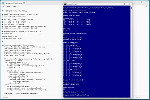
A good way to see where this article is headed is to take a look at the screenshot in Figure 1. The demo program loads a 200-item set of training data and a 40-item set of test data into memory. Next, the demo creates and trains a decision tree model using the DecisionTreeClassifier module from the scikit library.
 [Click on image for larger view.] Figure 1: Multi-Class Classification Using a scikit Decision Tree
After training, the model is applied to the training data and the test data. The model scores 84.00 percent accuracy (168 out of 200 correct) on the training data, and 77.50 percent accuracy (31 out of 40 correct) on the test data. The demo displays the model in pseudo-code.
The demo concludes by predicting the political leaning of a person who is male, age 35, from Nebraska and makes $55,000 per year. The prediction is [[0.0851 0.8298 0.0851]]. These are pseudo-probabilities and because the value at index [1] is largest, the predicted political type is moderate.
This article assumes you have intermediate or better skill with a C-family programming language, but doesn't assume you know much about decision trees or the scikit library. The complete source code for the demo program is presented in this article and the accompanying file download. The source code is also available online.
Installing the scikit Library
There are several ways to install the scikit library. I recommend installing the Anaconda Python distribution. Anaconda contains a core Python engine plus over 500 libraries that are (mostly) compatible with each other. I used Anaconda3-2020.02 which contains Python 3.7.6 and the scikit 0.22.1 version. The demo code runs on Windows 10 or 11.
Briefly, Anaconda is installed using a Windows self-extracting executable file. The setup process is mostly straightforward and takes about 15 minutes, with the help of my step-by-step instructions.
There are more up-to-date versions of Anaconda / Python / scikit library available. But because the Python ecosystem has hundreds of libraries, if you install the most recent versions of these libraries, you run a greater risk of library incompatibilities -- a big headache when working with Python.
The Data
The data is artificial and can be found here. There are 200 training items and 40 test items. The structure of data looks like:
1   0.24   1   0   0   0.2950   2
0   0.39   0   0   1   0.5120   1
1   0.63   0   1   0   0.7580   0
0   0.36   1   0   0   0.4450   1
1   0.27   0   1   0   0.2860   2
. . .
The tab-delimited fields are sex (0 = male, 1 = female), age (divided by 100), state (Michigan = 100, Nebraska = 010, Oklahoma = 001), income (divided by $100,000) and political leaning (conservative = 0, moderate = 1, liberal = 2). For decision tree classification, the variable to predict is most often ordinal-encoded (0, 1, 2 and so on) The numeric predictors do not need to be normalized to all the same range -- typically 0.0 to 1.0 or -1.0 to +1.0 -- but normalizing allows the dataset to be used by other machine learning techniques where normalization is necessary.
Dealing with categorical predictors is a bit subtle. I recommend that they should be one-hot encoded. For example, if there were five states instead of just three, the states would be encoded as 10000, 01000, 00100, 00010, 00001.
For ordinal predictors that have an implied order, it is possible to use ordinal encoding. For example, a predictor variable such as height with possible values "short", "medium", and "tall" could be encoded as short = 0, medium = 1, height = 2.
Understanding How a Decision Tree Works
The result of training a decision tree classifier is a set of if-then rules. The demo program rules look like:
|--- age <= 0.52
|   |--- age <= 0.30
|   |   |--- sex <= 0.50
|   |   |   |--- class: 0
|   |   |--- sex >  0.50
|   |   |   |--- class: 2
. . .
For example, a person who is age = 30 and who has sex = 1 (greater than 0.50) is predicted to be class 2 = liberal. Notice the somewhat awkward age <= 0.52 followed immediately by age <= 0.30. Redundant conditions like this are a characteristic of decision tree models.
Some of the rules may have a condition such as "if state2 < 0.5". Because the state of residence variable is encoded as Michigan = 100, Nebraska = 010, Oklahoma = 001, state2 is the third encoding value and the condition means the third encoding value is 0, and therefore the state is Michigan or Nebraska, or equivalently, not Oklahoma.
Starting with all 200 training items, the decision tree algorithm scans the data and finds the one value of the one predictor variable that splits the data into two sets in such a way that the most information is obtained. After the first split, the decision tree algorithm examines each of the two subsets of data and finds a predictor variable and a value that gives the most information. The process continues until a program-specified maximum tree depth is reached.
There are several algorithms to split data. The most common technique is called Gini impurity. The second most common splitting technique is called Shannon information gain. In practice, both techniques usually give similar results.
If a large tree depth value is used, it's possible to generate a very large tree that achieves 100 percent classification accuracy. But such a tree would overfit the training data and give poor accuracy on new, previously unseen data items.
The Demo Program
The complete demo program is presented in Listing 1. Notepad is my preferred code editor but most of my colleagues prefer one of the many excellent code editors that are available for Python. I indent my Python program using two spaces rather than the more common four spaces.
The program imports the NumPy library which contains numeric array functionality. The tree package contains the DecisionTree module has the key code for creating a multi-class decision tree. Notice the name of the root scikit module is sklearn rather than scikit.
Listing 1: Complete Demo Program
# people_politics_tree_sckit.py

# predict politics (0 = con, 1 = mod, 2 = lib)
# from sex, age, state, income

# sex  age    state    income   politics
#  0   0.27   0  1  0   0.7610   2
#  1   0.19   0  0  1   0.6550   0
# sex: 0 = male, 1 = female
# state: michigan = 100, nebraska = 010, oklahoma = 001
# politics: conservative, moderate, liberal

# Anaconda3-2020.02  Python 3.7.6  scikit 0.22.1
# Windows 10/11

import numpy as np
from sklearn import tree

# ---------------------------------------------------------

def main():
  # 0. get ready
  print("\nBegin scikit decision tree example ")
  print("Predict politics from sex, age, State, income ")
  np.random.seed(0)
  np.set_printoptions(precision=4, suppress=True)

  # 1. load data
  print("\nLoading data into memory ")
  train_file = ".\\Data\\people_train.txt"
  train_xy = np.loadtxt(train_file, usecols=range(0,7),
    delimiter="\t", comments="#",  dtype=np.float32)
  train_x = train_xy[:,0:6]
  train_y = train_xy[:,6].astype(int)

  test_file = ".\\Data\\people_test.txt"
  test_xy = np.loadtxt(test_file, usecols=range(0,7),
    delimiter="\t", comments="#",  dtype=np.float32)
  test_x = test_xy[:,0:6]
  test_y = test_xy[:,6].astype(int)

  print("\nTraining data:")
  print(train_x[0:4])
  print(". . . \n")
  print(train_y[0:4])
  print(". . . ")

  # 2. create and train
  md = 3
  print("\nCreating decision tree max_depth=" + \
    str(md))
  model = tree.DecisionTreeClassifier(max_depth=md)
  model.fit(train_x, train_y)
  print("Done ")

  # 3. evaluate
  acc_train = model.score(train_x, train_y)

  # 4a. visualize with built-in export_text()
  pseudo = tree.export_text(model,
    ["sex", "age",
    "state0", "state1", "state2",
    "income"])
  print("\nModel in pseudo-code: ")
  print(pseudo)

  # 4b. use built-in plot_tree()
  import matplotlib.pyplot as plt
  plt.figure(figsize=(14,8),
    tight_layout=True)  # w,h inches
  tree.plot_tree(model,
    feature_names=["sex", "age",
      "state0", "state1", "state2",
      "income"],
    class_names=["con", "mod", "lib"],
    fontsize=8)
  plt.show()

  # 5. use model
  print("\nPredict for: M 35 Nebraska $55K ")
  X = np.array([[0, 0.35, 0,1,0, 0.5500]],
    dtype=np.float32)
  probs = model.predict_proba(X)
  print("\nPrediction pseudo-probs: ")
  print(probs)

  politic = model.predict(X)
  print("\nPredicted class: ")
  print(politic)

  # 6. TODO: save model using pickle

  print("\nEnd scikit decision tree demo ")

if __name__ == "__main__":
  main()
The demo begins by setting the NumPy random seed:
def main():
  print("Predict politics from sex, age, State, income ")
  np.random.seed(0)
  np.set_printoptions(precision=4, suppress=True)
 . . .
Technically, setting the random seed value isn't necessary, but doing so helps you to get reproducible results in most situations. The set_printoptions() function formats NumPy arrays to four decimals without using scientific notation.
Loading the Training and Test Data
The demo program loads the training data into memory using these statements:
  # 1. load data
  print("Loading data into memory ")
  train_file = ".\\Data\\people_train.txt"
  train_xy = np.loadtxt(train_file, usecols=range(0,7),
    delimiter="\t", comments="#",  dtype=np.float32)
  train_x = train_xy[:,0:6]
  train_y = train_xy[:,6].astype(int)
This code assumes the data files are stored in a directory named Data. There are many ways to load data into memory. I prefer using the NumPy library loadtxt() function, but a common alternative is the Pandas library read_csv() function.
The code reads all 200 lines of training data (columns 0 to 6 inclusive) into a matrix named train_xy and then splits the data into a matrix of predictor values and a vector of target gender values. The colon syntax means "all rows".
The 40-item test data is read into memory in the same way as the training data:
  test_file = ".\\Data\\people_test.txt"
  test_xy = np.loadtxt(test_file, usecols=range(0,7),
    delimiter="\t", comments="#",  dtype=np.float32)
  test_x = test_xy[:,0:6]
  test_y = test_xy[:,6].astype(int)
The demo program prints the first four predictor items and the first four target politics values:
  print("Training data:")
  print(train_x[0:4])
  print(". . . \n")
  print(train_y[0:4])
  print(". . . ")
In a non-demo scenario, you might want to display all the training data and all the test data to verify the data has been read properly.
Creating and Training the Model
Creating and training the multi-class classification decision tree model is simultaneously simple and complicated:
  # 2. create and train
  md = 3
  print("Creating decision tree max_depth=" + str(md))
  model = tree.DecisionTreeClassifier(max_depth=md)
  model.fit(train_x, train_y)
  print("Done ")
Like most scikit models, the DecisionTreeClassifier class has a lot of parameters:
DecisionTreeClassifier(*, criterion='gini', splitter='best', max_depth=None, min_samples_split=2, min_samples_leaf=1, min_weight_fraction_leaf=0.0, max_features=None, random_state=None, max_leaf_nodes=None, min_impurity_decrease=0.0, class_weight=None, ccp_alpha=0.0)
When working with scikit, you'll spend most of your time reading the documentation and trying to figure out what each parameter does. The most important parameter to tune is max_depth. The random_state parameter is a seed value for the model internal random number generator.
Notice that 'gini' is the default splitting algorithm. In most situations, the default values of the other parameters can be used. After everything has been prepared, the model is trained using the fit() method. Easy.
Evaluating the Trained Model
The demo computes the accuracy of the trained model like so:
  # 3. evaluate
  acc_train = model.score(train_x, train_y)
  print("Accuracy on train = %0.4f " % acc_train)
  acc_test = model.score(test_x, test_y)
  print("Accuracy on test = %0.4f " % acc_test)
The score() function computes a simple accuracy which is just the number of correct predictions divided by the total number of predictions. However, for classification problems you often want additional evaluation metrics. One common technique is to display a confusion matrix that shows details of the counts of which classes have been incorrectly predicted. For example:
  # display confusion matrix
  from sklearn.metrics import confusion_matrix
  y_predicteds = model.predict(test_x)
  cm = confusion_matrix(test_y, y_predicteds)
  print("Confusion matrix: ")
  print(cm)
The result for the demo program is:
  [[6  4  1]
   [1 13  0]
   [2  1 12]]
The 4 value means that there are 4 data items that have actual class 0 but are predicted class 1. A scikit raw confusion matrix is a bit difficult to interpret. But it's easy to write a program-defined function that adds labels to the matrix.
Visualizing the Decision Tree
The demo program displays the trained decision tree rules in pseudo-code like so:
  # 4a. visualize using built-in export_text()
  pseudo = tree.export_text(model,
    ["sex", "age",
    "state0", "state1", "state2",
    "income"])
  print("Model in pseudo-code: ")
  print(pseudo)
The export_text() function is relatively new to scikit. Before export_text() as added, it was necessary to write a custom function to display a tree in pseudo-code. The demo program contains an example of such a custom function.
It is also possible to display a decision tree graphically:
  # 4b. use built-in plot_tree()
  import matplotlib.pyplot as plt
  plt.figure(figsize=(14,8),
    tight_layout=True)  # w,h inches
  tree.plot_tree(model,
    feature_names=["sex", "age",
      "state0", "state1", "state2",
      "income"],
    class_names=["con", "mod", "lib"],
    fontsize=8)
  plt.show()
The result in shown in Figure 2. Because decision trees can be very large, it's often necessary to adjust the figsize() and fontsize() parameters.
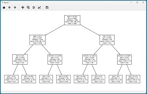 [Click on image for larger view.] Figure 2: Decision Tree Displayed Graphically
The ability to display a decision tree model makes trees somewhat interpretable. This is an advantage of tree classifiers compared to neural networks.
Using the Trained Model
The demo uses the trained model like so:
  # 5. use model
  print("Predict for: M 35 Nebraska $55K ")
  X = np.array([[0, 0.35, 0,1,0, 0.5500]],
    dtype=np.float32)
  probs = model.predict_proba(X)
  print("Prediction pseudo-probs: ")
  print(probs)
Because the decision tree model was trained using normalized and encoded data, the x-input must be normalized and encoded in the same way. Notice the double square brackets on the x-input. The predict_proba() method expects a matrix rather than a vector. The result of the proba() method ("probability array") is a vector of pseudo-probabilities that sum to 1. If the class-to-predict is ordinal encoded, the index of the largest value corresponds to the predicted class.
The demo concludes by predicting the political type directly by using the predict() method:
  politic = model.predict(X)
  print("Predicted class: ")
  print(politic)
The result is an array with one value -- [1] -- rather than the scalar value 1 because the predict() method accepts a matrix of predictor values instead of a single vector of values. To display the predicted class as a string you can write code like:
classes = model.predict(X)  # vector with one value: [1]
idx = classes[0]            # the value: 1
labels = ["conservative", "moderate", "liberal"]
predicted = labels[idx]     # moderate
print(predicted)
Wrapping Up
The demo program uses the scikit DecisionTree module for multi-class classification. An alternative approach is to use the scikit MLPClassifier module (multi-layer perceptron). The MLPClassifier module implements a neural network with one (shallow) or more (deep) hidden layers. Decision trees are useful for relatively small datasets that have a relatively simple underlying structure, and when the trained model must be easily interpretable. Neural networks are useful for large datasets with complex structures, but neural models are not easy to interpret. Because the scikit library is so easy to use, it's common to try both approaches.