The Data Science Lab

Gaussian Process Regression from Scratch Using C#

GPR works well with small datasets and generates a metric of confidence of a predicted result, but it's moderately complex and the results are not easily interpretable, says Dr. James McCaffrey of Microsoft Research in this full-code tutorial.

• By James McCaffrey
• 09/15/2023

The goal of a machine learning regression problem is to predict a single numeric value. For example, you might want to predict the monthly rent of an apartment in a particular city based on the square footage, number of bedrooms, local tax rate and so on.

There are roughly a dozen major regression techniques, and each technique has several variations. The most common techniques include linear regression, linear ridge regression, k-nearest neighbors regression, kernel ridge regression, Gaussian process regression, decision tree regression and neural network regression. Each technique has pros and cons. This article explains how to implement Gaussian process regression (GPR) from scratch, using the C# language. Compared to other regression techniques, GPR works well with small datasets, and generates a metric of confidence of a predicted result. However, GPR is moderately complex, and the results are not easily interpretable.

Gaussian process regression is a sophisticated technique that uses what is called the kernel trick to deal with complex non-linear data, and L2 regularization to avoid model overfitting where a model predicts training data well but predicts new, previously unseen data poorly. A distinguishing characteristic of GPR is that it produces a predicted value, but also a standard deviation which is a measure of prediction uncertainty/confidence. For example, a GPR prediction might be, "y = 0.5123 with standard deviation 0.06," which can loosely be interpreted to mean that 0.5123 plus or minus 0.06 will capture the true y value roughly 68 percent of the time if a series of simulations were performed.

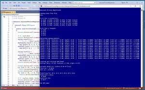
A good way to see where this article is headed is to take a look at the screenshot of a demo program in Figure 1. The demo program uses synthetic data that was generated by a 6-10-1 neural network with random weights. There are six predictor variables which have values between -1.0 and +1.0, and a target variable to predict which is a value between 0.0 and 1.0. There are 200 training items and 40 test items. The data looks like:

-0.1660, 0.4406, -0.9998, -0.3953, -0.7065, -0.8153, 0.9386
-0.2065, 0.0776, -0.1616,  0.3704, -0.5911,  0.7562, 0.4374
-0.9452, 0.3409, -0.1654,  0.1174, -0.7192, -0.6038, 0.8437
 0.7528, 0.7892, -0.8299, -0.9219, -0.6603,  0.7563, 0.8765
. . .

The demo program creates a GPR model using the training data. The model uses three parameters. A theta parameter is set to 0.50 and a length scale parameter is set to 2.00. The theta and length scale parameters control the model's internal radial basis function (RBF), which is a key component of the kernel mechanism. An alpha parameter is set to 0.01 and is used by the L2 regularization mechanism of GPR. The values of theta, length scale and alpha were determined by using a grid search and picking the values that gave balanced model accuracy and model root mean squared error.

After the GPR model is created, it is applied to the training and test data. The model scores 0.8650 accuracy on the training data (173 out of 200 correct) and 0.8250 accuracy on the test data (33 out of 40 correct). A correct prediction is defined as one that is within 10 percent of the true target value.

The demo program concludes by making a prediction for a new, previously unseen data item x = (0.1, 0.2, 0.3, 0.4, 0.5, 0.6). The predicted y value is 0.5694 with standard deviation 0.0377.

This article assumes you have intermediate or better programming skill but doesn't assume you know anything about Gaussian process regression. The demo is implemented using C# but you should be able to refactor the code to a different C-family language if you wish.

Understanding Gaussian Process Regression
I suspect that one of the reasons why Gaussian process regression is not used as often as other regression techniques is that GPR is very intimidating from a mathematical perspective. So bear with me. There are hundreds of web pages and many hours of videos that explain GPR. The mere fact that there are so many explanations available is an indirect indication of the complexity of the technique.

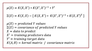
The key equations for GPR are shown in Figure 2. There are many variations of GPR equations so the ones shown here may not look like those in other references unless you examine them carefully. The mathematical derivation of these equations is complex and is outside the scope of this article.

Two of the key ideas in GPR are kernel functions and kernel matrices. A kernel function accepts two vectors and returns a number that is a measure of their similarity. There are many different kernel functions, and there are several variations of each type of kernel function. The most commonly used kernel function (in the projects I've been involved with, at any rate) is the radial basis function (RBF), also called the squared exponential function.

The form of the composite RBF function used by the demo program is rbf(x1, x2) = theta * exp(-1 * ||x1 - x2|| / (2 * s^2)) where x1 and x2 are two vectors, ||x1 - x2|| is the squared Euclidean distance between x1 and x2, theta is a constant, and s is a constant called the length scale.

Suppose x1 = (0.1, 0.5, 0.7) and x2 = (0.4, 0.3, 0.6) and theta = 3.0 and s = 1.0. The squared Euclidean distance, ||x1 - x2||, is the sum of the squared differences of the vector elements: (0.1 - 0.4)^2 + (0.5 - 0.3)^2 + (0.7 - 0.6)^2 = 0.09 + 0.04 + 0.01 = 0.14. Therefore,

rbf(x1, x2) = 3.0 * exp( -1 * 0.14 / (2 * 1.0^2) ) 
            = 3.0 * exp(-0.14 / 2)
            = 3.0 * exp(-0.07) 
            = 3.0 * 0.9324
            = 2.7972

The theta value is often considered a separate kernel function without any parameters, called the Constant Kernel. So the composite kernel function used by the demo program can be interpreted as k(x1, x2) = Constant Kernel * RBF(x1, x2), where Constant Kernel = 3.0 and RBF(x1, x2) = exp( -1 * ||x1 - x2|| / (2 * s^2) ).

If two vectors are identical (maximum similarity), their non-composite RBF value is 1.0. As the two vectors decrease in similarity, the RBF value approaches, but never quite reaches, 0.0.

The demo program uses the composite version of RBF because it's the version used by default by the scikit-learn code library GaussianProcessRegressor module. Another common version of a plain RBF (not composite) is rbf(x1, x2) = exp( -1 * gamma * ||x1 - x2|| ) where gamma is a constant.

A kernel matrix is best explained by example. Suppose there are just three training vectors, X' = x0, x1, x2. Each vector has two or more predictor variables, six in the case of the demo program. The K(X', X') kernel matrix is 3 x 3 with these entries:

[0]  rbf(x0, x0)  rbf(x0, x1)  rbf(x0, x2)
[1]  rbf(x1, x0)  rbf(x1, x1)  rbf(x1, x2) 
[2]  rbf(x2, x0)  rbf(x2, x1)  rbf(x2, x2) 
          [0]          [1]          [2]

Notice that the entries on the diagonal will be 1.0 (for a non-composite RBF function, or a composite RBF function with theta = 1.0) and that entries off the diagonal are a measure of training vector similarity, or equivalently, a measure of dispersion. This is the format of a classical statistics covariance matrix.

Expressed in an informal mathematical style, the GPR prediction equations are:

mean(X) = K(X, X') * inv(K(X', X')) * Y'
covar(X) = K(X, X) - [K(X, X') * inv(K(X', X')) * tr(K(X, X'))]

Here X represents a matrix of x values to predict, where each row is a vector of predictor values. Although it's possible to write GPR equations relative to a single input x vector, it's common to express everything as matrices.

The mean(X) is a matrix of the predicted values. The covar(X) is a matrix of the prediction covariances.

The X' term is a matrix of the training data inputs. The Y' term is a matrix of training data target values. The K() is a matrix of kernel values so K(X, X') is a matrix of values that compare each input vector with each training vector. K(X', X') is a matrix of kernel function values that compare each training vector with all possible combinations of themselves. The K(X', X') is called the covariance matrix. The inv() represents matrix inverse, the tr() represents matrix transpose, * represents matrix multiplication, and - represents matrix subtraction. Whew!

From a practical point of view, there are two key takeaways. First, in order to make a prediction using GPR, you need all training data (to compute the K(X', X') and K(X, X') matrices). Second, because of the inv(K(X', X')) term, if there are n training items, then the inverse of a matrix with size n x n is computed, and so GPR does not scale well to problems with huge datasets.

The matrix inverse function can fail for several reasons. GPR adds a small constant, usually called alpha or noise or lambda, to the diagonal of the K(X', X') covariance matrix before applying the inverse() operation. This helps to prevent inverse() from failing and is called conditioning the matrix. Adding an alpha/noise to the covariance matrix also introduces L2 regularization ("ridge"), which deters model overfitting.

Because GPR adds the same small constant alpha/noise value to each column of the K(X', X') matrix, the predictor data should be normalized to roughly the same scale. The three most common normalization techniques are divide-by-constant, min-max and z-score. I recommend divide-by-constant. For example, if one of the predictor variables is a person's age, you could divide all ages by 100 so that the normalized age values are all between 0.0 and 1.0.

The demo program uses a standard technique called Crout's decomposition to invert the K(X', X') covariance matrix. Because K(X', X') is a symmetric, positive definite matrix, it's possible to use a specialized, slightly more efficient technique called Cholesky decomposition. The difference of a few milliseconds isn't usually important in most machine learning scenarios. See my article, "Matrix Inversion Using Cholesky Decomposition With C#."

Overall Program Structure
I used Visual Studio 2022 (Community Free Edition) for the demo program. I created a new C# console application and checked the "Place solution and project in the same directory" option. I specified .NET version 6.0. I named the project GaussianProcessRegression. I checked the "Do not use top-level statements" option to avoid the confusing program entry point shortcut syntax.

The demo has no significant .NET dependencies, and any relatively recent version of Visual Studio with .NET (Core) or the older .NET Framework will work fine. You can also use the Visual Studio Code program if you like.

After the template code loaded into the editor, I right-clicked on file Program.cs in the Solution Explorer window and renamed the file to the slightly more descriptive GPRProgram.cs. I allowed Visual Studio to automatically rename class Program.

The overall program structure is presented in Listing 1. The GPRProgram class houses the Main() method, which has all the control logic. The GPR class houses all the Gaussian process regression functionality such as the Predict() and Accuracy() methods. The Utils class houses all the matrix helper functions such as MatLoad() to load data into a matrix from a text file, and MatInverse() to find the inverse of a matrix.

Listing 1: Overall Program Structure

using System;
using System.IO;

namespace GaussianProcessRegression
{
  internal class GPRProgram
  {
    static void Main(string[] args)
    {
      Console.WriteLine("Gaussian Process Regression ");

      // 1. load data
      // 2. explore alpha, theta, lenScale hyperparameters
      // 3. create and train model
      // 4. evaluate model
      // 5. use model for previously unseen data
      
      Console.WriteLine("End GPR demo ");
      Console.ReadLine();
    } // Main()
  } // Program

  public class GPR
  {
    public double theta = 0.0;
    public double lenScale = 0.0;
    public double noise = 0.0;
    public double[][] trainX;
    public double[] trainY;
    public double[][] invCovarMat;

    public GPR(double theta, double lenScale,
      double noise, double[][] trainX, double[] trainY) { . . }
    
    public double[][] ComputeCovarMat(double[][] X1,
      double[][] X2) { . . }
    
    public double KernelFunc(double[] x1, double[] x2) { . . }
    
    public double[][] Predict(double[][] X) { . . }

    public double Accuracy(double[][] dataX, double[] dataY,
      double pctClose) { . . }
    
    public double RootMSE(double[][] dataX,
      double[] dataY) { . . }
  } // class GPR

  public class Utils
  {
    public static double[][] VecToMat(double[] vec,
      int nRows, int nCols) { . . }
    
    public static double[][] MatCreate(int rows,
      int cols) { . . }
    
    public static double[] MatToVec(double[][] m) { . . }
    
    public static double[][] MatProduct(double[][] matA,
      double[][] matB) { . . }
    
    public static double[][] MatTranspose(double[][] m) { . . }
    
    public static double[][] MatDifference(double[][] matA,
      double[][] matB) { . . }
    
    // -------

    public static double[][] MatInverse(double[][] m) { . . }
    
    static int MatDecompose(double[][] m,
      out double[][] lum, out int[] perm) { . . }

    static double[] Reduce(double[][] luMatrix,
      double[] b) { . . }
    
    // -------

    static int NumNonCommentLines(string fn,
      string comment) { . . }
    
    public static double[][] MatLoad(string fn,
      int[] usecols, char sep, string comment) { . . }
    
    public static void MatShow(double[][] m,
      int dec, int wid) { . . }
    
    public static void VecShow(int[] vec, int wid) { . . }
    
    public static void VecShow(double[] vec,
      int dec, int wid) { . . }
  } // class Utils
} // ns

Although the demo program is long, the majority of the code is in the helper Utils class. The demo program begins by loading the synthetic training data into memory:

Console.WriteLine("Loading data from file ");
string trainFile =
  "..\\..\\..\\Data\\synthetic_train_200.txt";
double[][] trainX = Utils.MatLoad(trainFile,
  new int[] { 0, 1, 2, 3, 4, 5 }, ',', "#");
double[] trainY = Utils.MatToVec(Utils.MatLoad(trainFile,
  new int[] { 6 }, ',', "#"));

The code assumes the data is located in a subdirectory named Data. The call to the MatLoad() utility function specifies that the data is comma delimited and uses the '#' character to identify lines that are comments. The test data is loaded into memory in the same way:

string testFile =
  "..\\..\\..\\Data\\synthetic_test_40.txt";
double[][] testX = Utils.MatLoad(testFile,
  new int[] { 0, 1, 2, 3, 4, 5 }, ',', "#");
double[] testY = Utils.MatToVec(Utils.MatLoad(testFile,
  new int[] { 6 }, ',', "#"));
Console.WriteLine("Done ");

Next, the demo displays the first four training predictor values and target values:

Console.WriteLine("First four X predictors: ");
for (int i = 0; i < 4; ++i)
  Utils.VecShow(trainX[i], 4, 8);
Console.WriteLine("\nFirst four y targets: ");
for (int i = 0; i < 4; ++i)
  Console.WriteLine(trainY[i].ToString("F4").PadLeft(8));

In a non-demo scenario you'd probably want to display all training and test data to make sure it was loaded correctly.

Creating and Training the GPR Model
After loading the training data, the demo uses a grid search to find good values for the RBF theta and length scale parameters, and the alpha/noise parameter. In pseudo-code:

  set candidate alpha, theta, scale values
  for-each alpha value
    for-each theta value
      for-each length scale value
        create/train GPR model using alpha, theta, scale
        evaluate model accuracy and RMSE
      end-for
    end-for
  end-for

Finding good hyperparameter values is somewhat subjective. The idea is to balance accuracy, which is a crude metric but ultimately the one you're usually interested in, with root mean squared error (RMSE), which is a granular metric but one that can be misleading.

After determining good model parameter values, the GPR model is simultaneously created and trained:

Console.WriteLine("Creating and training GPR model ");
double theta = 0.50;    // "constant kernel"
double lenScale = 2.0;  // RBF parameter
double alpha = 0.01;    // noise
Console.WriteLine("Setting theta = " +
  theta.ToString("F2") + ", lenScale = " +
  lenScale.ToString("F2") + ", alpha = " +
  alpha.ToString("F2"));

GPR model = new GPR(theta, lenScale, alpha,
  trainX, trainY);  // create and train

The GPR constructor uses the training data to create the inverse of the K(X', X') covariance matrix for use by the Predict() method.

GPR models are different from many other regression techniques because there is no explicit training. For example, a neural network regression model uses training data to create what is essentially a very complicated prediction equation, after which the training data is no longer needed. GPR needs all training data to make a prediction, therefore, the training data is passed to the GPR constructor. An alternative API design is to use an explicit Train() method that stores the training data and computes the inverse of the covariance matrix for later use by the Predict() method:

// alternative API design
GPR model = new GPR(theta: 0.5, lenScale: 2.0, noise: 0.01);
model.Train(trainX, trainY);  // stores data, computes inverse

This approach is used by several machine learning libraries, notably scikit-learn, to provide an API that is consistent across all regression techniques in the library.

Evaluating and Using the GPR Model
After the GPR model is created and implicitly trained, the demo evaluates the model using these statements:

Console.WriteLine("Evaluate model acc" +
  " (within 0.10 of true)");
double trainAcc = model.Accuracy(trainX, trainY, 0.10);
double testAcc = model.Accuracy(testX, testY, 0.10);
Console.WriteLine("Train acc = " +
  trainAcc.ToString("F4"));
Console.WriteLine("Test acc = " +
  testAcc.ToString("F4"));

Because there's no inherent definition of regression accuracy, it's necessary to implement a program-defined method. How close a predicted value must be to the true value in order to be considered a correct prediction, will vary from problem to problem.

The demo concludes by using the trained model to predict for x = (0.1, 0.2, 0.3, 0.4, 0.5, 0.6) using these statements:

Console.WriteLine("Predicting for (0.1, 0.2, 0.3," + 
  " 0.4, 0.5, 0.6) ");
double[][] X = Utils.MatCreate(1, 6);
X[0] = new double[] { 0.1, 0.2, 0.3, 0.4, 0.5, 0.6 };

double[][] results = model.Predict(X);
Console.WriteLine("Predicted y value: ");
double[] means = results[0];
Utils.VecShow(means, 4, 8);
Console.WriteLine("Predicted std: ");
double[] stds = results[1];
Utils.VecShow(stds, 4, 8);

Recall that the Predict() method is expecting a matrix of input values, not just a single vector. Therefore, the demo creates an input matrix with one row and six columns, but just uses the first row at [0].

The return value from Predict() is an array with two cells. The first cell of the return at index [0] holds another array of predicted y values, one for each row of the input matrix, which in this case is just one row. The second cell of the return at index [1] holds an array of standard deviations, one for each prediction.

You should interpret the standard deviations of the Predict() method conservatively. Gaussian process regression makes several assumptions about the Gaussian distribution of the source data, which may not be completely correct. For example, if you have a predicted y with value 0.50 and a standard deviation of 0.06, it's usually better to just report these values rather than use the standard deviation to construct a classical statistics confidence interval along the lines of, "predicted y = 0.50 with a 95% confidence interval of plus or minus 1.96 * 0.06."

Wrapping Up
Implementing Gaussian process regression from scratch requires significant effort. But doing so allows you to customize the system for unusual scenarios, makes it easy to integrate the prediction code with other systems, and removes a significant external dependency.

The GPR system presented in this article uses a hard-coded composite radial basis function as the kernel function. There are about a dozen other common kernel functions such as polynomial, Laplacian and sigmoid. You can experiment with these kernel functions but there are no good rules of thumb for picking a function based on the nature of your data.

The demo program uses predictor variables that are strictly numeric. GPR can handle categorical data by using one-hot encoding. For example, if you had a predictor variable color with possible values red, blue, green, you could encode red = (1, 0, 0), blue = (0, 1, 0), green = (0, 0, 1).

A technique closely related to Gaussian process regression is kernel ridge regression (KRR), which I explain in last month's article, "Kernel Ridge Regression Using C#." KRR starts with what appear to be different math assumptions than GPR, but KRR ends up with the same prediction equation as GPR. However, KRR has less restrictive assumptions which do not allow KRR to produce a prediction standard deviation -- KRR produces just a point estimate without a standard deviation.

• Get Code Download