The Data Science Lab

Data Anomaly Detection Using a Neural Autoencoder with C#

Dr. James McCaffrey of Microsoft Research tackles the process of examining a set of source data to find data items that are different in some way from the majority of the source items.

• By James McCaffrey
• 04/15/2024

Data anomaly detection is the process of examining a set of source data to find data items that are different in some way from the majority of the source items. There are many different types of anomaly detection techniques. This article explains how to use a neural autoencoder implemented using raw C# to find anomalous data items.

Compared to other anomaly detection techniques, using a neural autoencoder is theoretically the most powerful approach. But using an autoencoder can be a difficult technique to fine-tune because you must find the values for several hyperparameters -- specifically, number of hidden nodes, maximum iterations, batch size, and learning rate -- using trial and error guided by experience.

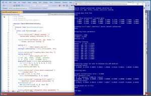
A good way to see where this article is headed is to take a look at the screenshot of a demo program in Figure 1. The demo uses a synthetic dataset that has 240 items. The raw data looks like:

F  24  michigan  29500.00  liberal
M  39  oklahoma  51200.00  moderate
F  63  nebraska  75800.00  conservative
M  36  michigan  44500.00  moderate
F  27  nebraska  28600.00  liberal
. . .

Each line of data represents a person. The fields are sex (male, female), age, State (Michigan, Nebraska, Oklahoma), income, and political leaning (conservative, moderate, liberal). Notice that neural autoencoders can deal with any type of data: Boolean, integer, categorical/text, and floating point. The source data has been normalized and encoded, and looks like:

1, 0.24, 1, 0, 0, 0.2950, 0, 0, 1
0, 0.39, 0, 0, 1, 0.5120, 0, 1, 0
1, 0.63, 0, 1, 0, 0.7580, 1, 0, 0
0, 0.36, 1, 0, 0, 0.4450, 0, 1, 0
1, 0.27, 0, 1, 0, 0.2860, 0, 0, 1
. . .

Preparing the raw source data usually requires most of the time and effort for anomaly detection using a neural autoencoder, or any other type of anomaly detection. The demo program begins by loading the normalized and encoded data from text file into memory.

The demo instantiates a 9-6-9 neural autoencoder that has tanh() hidden layer activation and identity() output layer activation. Then, training parameters are set to maxEpochs = 1000, lrnRate = 0.010, and batSize = 10. The autoencoder Train() method is called, and progress is monitored every 100 epochs:

Starting training
epoch:    0  MSE = 1.6188
epoch:  100  MSE = 0.0028
epoch:  200  MSE = 0.0013
. . .
epoch:  900  MSE = 0.0006
Done

The MSE (mean squared error) values decrease which indicates that training is working properly -- something that doesn't always happen.

The trained neural autoencoder is subjected to a sanity check by predicting the output for the second person in the dataset: a person who is male, age 39, lives in Oklahoma, makes $51,200 and is politically moderate. The computed output is (0.00390, 0.39768, -0.00035, -0.00252, 1.00286, 0.50118, -0.00225, 1.00290, -0.00065) which is reasonable, as will be explained shortly.

The trained neural autoencoder model is used to scan all 240 data items. The data item that has the largest reconstruction error is (M, 36, nebraska, $53000.00, liberal), which has encoded and normalized form (0.00000, 0.36000, 0.00000, 1.00000, 0.00000, 0.53000, 0.00000, 0.00000, 1.00000). The predicted output is (-0.00122, 0.40366, -0.00134, 0.99657, 0.00477, 0.49658, 0.01607, -0.01048, 0.99440). This indicates that the anomalous data item has an age value that's a bit too small (actual 36 versus a predicted of 40) and an income value that's a bit too large (actual $53,000 versus a predicted of $49,658).

The demo concludes by saving the trained autoencoder model to file in case it's needed later. At this point, in a non-demo scenario, the anomalous data item would be examined further to try and determine why the autoencoder model flagged the item as anomalous.

This article assumes you have intermediate or better programming skill but doesn't assume you know anything about neural autoencoders. The demo is implemented using C# but you should be able to refactor the demo code to another C-family language if you wish, but it would require a significant effort.

The source code for the demo program is too long to be presented in its entirety in this article. The complete code and data are available in the accompanying file download, and are also available online.

Understanding Neural Autoencoders
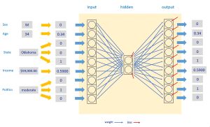
The diagram in Figure 2 illustrates a neural autoencoder. The autoencoder has the same number of inputs and outputs (9) as the demo program, but for simplicity the illustrated autoencoder has architecture 9-2-9 (just 2 hidden nodes) instead of the 9-6-9 architecture of the demo autoencoder.

A neural autoencoder is essentially a complex mathematical function that predicts its input. All input must be numeric so categorical data must be encoded. Although not theoretically necessary, for practical reasons, numeric input should be normalized so that all values have roughly the same range, typically between -1 and +1.

Each small blue arrow represents a neural weight, which is just a number, typically between about -2 and +2. Weights are sometimes called trainable parameters. The small red arrows are special weights called biases. The 9-2-9 autoencoder in the diagram has (9 * 2) + (2 * 9) = 36 weights, and 2 + 9 = 11 biases.

The values of the weights and biases determine the values of the output nodes. Finding the values of the weights and biases is called training the model. Put another way, training a neural autoencoder finds the values of the weights and biases so that the output values closely match the input values.

After training, all data items are fed to the trained model, and the output is compared to the input. The difference between the input vector and the output vector is called the reconstruction error. A large reconstruction error indicates that a data item does not fit the model well, and so the item is anomalous in some way.

Normalizing and Encoding Source Data
In practice, normalizing numeric data and encoding categorical data is often tedious and time-consuming. There are three common normalization techniques: divide-by-constant, min-max, and z-score. The demo program uses divide-by-constant. The raw age values are divided by 100, and the raw income values are divided by 100,000. There is strong, but currently unpublished, research evidence that indicates divide-by-constant normalization works well for neural systems. Briefly, compared to min-max and z-score normalization, divide-by-constant preserves the sign of the raw data, zero values are preserved, the normalized values are easy to interpret, and it's easy to normalize a train-test split of the data.

To encode categorical data, it's best to use what's called one-hot encoding. For the State predictor variable with 3 possible values, the encoding is Michigan = 100, Nebraska = 010, Oklahoma = 001. If the State variable had an additional possible value, say Pennsylvania, the encoding would be Michigan = 1000, Nebraska = 0100, Oklahoma = 0010, Pennsylvania = 0001. The order used in one-hot encoding is arbitrary.

A tricky topic is encoding binary (two possible values) predictor variables, such as the sex variable in the demo. Theoretically, it's best to encode as minus-one-plus-one, for example male = -1, female = +1. However, zero-one encoding is often used for binary predictors, for example, male = 0, female = 1. In practice, minus-one-plus-one encoding and zero-one encoding work equally well. The demo uses zero-one encoding for the sex variable.

The demo program assumes that the raw data has been normalized and encoded in a preprocessing step. It's possible to programmatically normalize and encode raw data on the fly, but in my opinion, this approach adds complexity to the system without a big benefit.

The Demo Program
I used Visual Studio 2022 (Community Free Edition) for the demo program. I created a new C# console application and checked the "Place solution and project in the same directory" option. I specified .NET version 8.0. I named the project NeuralNetworkAutoAnomaly. I checked the "Do not use top-level statements" option to avoid the program entry point shortcut syntax.

The demo has no significant .NET dependencies and any relatively recent version of Visual Studio with .NET (Core) or the older .NET Framework will work fine. You can also use the Visual Studio Code program if you like.

After the template code loaded into the editor, I right-clicked on file Program.cs in the Solution Explorer window and renamed the file to the slightly more descriptive NeuralAnomalyProgram.cs. I allowed Visual Studio to automatically rename class Program.

The overall program structure is presented in Listing 1. All the control logic is in the Main() method. All of the neural autoencoder functionality is in a NeuralNetwork class. A Utils class holds functions to load data from file to memory, and functions to display vectors and matrices.

Listing 1: Overall Program Structure

using System;
using System.IO;
using System.Collections.Generic;

namespace NeuralNetworkAutoAnomaly
{
  internal class NeuralAnomalyProgram
  {
    static void Main(string[] args)
    {
      Console.WriteLine("Neural network " +
        "autoencoder anomaly detection C# ");

      // load data
      // create autoencoder
      // train autoencoder
      // analyze data using autoencoder
      // save trained autoencoder

      Console.WriteLine("End demo ");
      Console.ReadLine();
    } // Main

  } // Program

  // --------------------------------------------------------

  public class NeuralNetwork
  {
    private int ni; // number input nodes
    private int nh;
    private int no;

    private double[] iNodes;
    private double[][] ihWeights; // input-hidden
    private double[] hBiases;
    private double[] hNodes;

    private double[][] hoWeights; // hidden-output
    private double[] oBiases;
    private double[] oNodes;  // single val as array

    // gradients
    private double[][] ihGrads;
    private double[] hbGrads;
    private double[][] hoGrads;
    private double[] obGrads;

    private Random rnd;

    public NeuralNetwork(int numIn, int numHid,
      int numOut, int seed) { . . }
 
    private void InitWeights() { . . }
    public void SetWeights(double[] wts) { . . }
    public double[] GetWeights() { . . }

    public double[] ComputeOutput(double[] x) { . . }
    private static double HyperTan(double x) { . . }
    private static double Identity(double x) { . . }
    private void ZeroOutGrads() { . . }
    private void AccumGrads(double[] y) { . . }
    private void UpdateWeights(double lrnRate) { . . }

    public void Train(double[][] dataX, double[][] dataY,
      double lrnRate, int batSize, int maxEpochs) { . . }

    public void Analyze(double[][] dataX, 
      string[] rawFileArray) { . . }
 
    private void Shuffle(int[] sequence) { . . }
    public double Error(double[][] dataX, 
      double[][] dataY) { . . }
    public void SaveWeights(string fn) { . . }
    public void LoadWeights(string fn) { . . }
  }

  // --------------------------------------------------------

  public class Utils
  {
    public static double[][] VecToMat(double[] vec,
      int rows, int cols) { . . }
    public static double[][] MatCreate(int rows,
      int cols) { . . }
    public static string[] FileLoad(string fn,
      string comment) { . . }
    public static double[][] MatLoad(string fn,
      int[] usecols, char sep, string comment) { . . }
    public static double[] MatToVec(double[][] m)
      { . . }
    public static void MatShow(double[][] m,
      int dec, int wid) { . . }
    public static void VecShow(int[] vec,
      int wid) { . . }
    public static void VecShow(double[] vec,
      int dec, int wid, bool newLine) { . . }
  }
} // ns

The demo program is complex. However, the only code you'll need to modify is the calling code in the Main() method. The demo starts by loading the raw data into memory:

string rf =
  "..\\..\\..\\Data\\people_raw.txt";
string[] rawFileArray = Utils.FileLoad(rf, "#");

Console.WriteLine("Loading data from file ");
string dataFile =
  "..\\..\\..\\Data\\people_all.txt";
// sex, age,  State,  income,  politics
//  0   0.32  1 0 0   0.65400  0 0 1
double[][] dataX = Utils.MatLoad(dataFile,
  new int[] { 0, 1, 2, 3, 4, 5, 6, 7, 8 },
  ',', "#"); // 240 items

The people_raw.txt file is read into memory as an array of type string. The arguments to the MatLoad() function mean load columns 0 through 8 inclusive of the comma-delimited file, where lines beginning with # indicate a comment. The return value is an array-of-arrays style matrix.

Part of the normalized and encoded data is displayed as a sanity check:

Console.WriteLine("First three normalized" +
  " / encoded data: ");
for (int i = 0; i < 3; ++i)
  Utils.VecShow(dataX[i], 4, 9, true);

The arguments to VecShow() means display using 4 decimals, with field width 9, and show indices.

Creating and Training the Autoencoder
The demo program creates a 9-6-9 autoencoder using these statements:

Console.WriteLine("Creating 9-6-9 tanh()" +
  " identity() neural network autoencoder ");
NeuralNetwork nn =
  new NeuralNetwork(9, 6, 9, seed: 0);
Console.WriteLine("Done ");

The number of input nodes and output nodes, 9 in the case of the demo, is entirely determined by the normalized source data. The number of hidden nodes, 6 in the demo, is a hyperparameter that must be determined by trial and error. If too few hidden nodes are used, the autoencoder doesn't have enough power to model the source data well. If too many hidden nodes are used, the autoencoder will essentially memorize the source data -- overfitting the data, and the model won't find anomalies.

The seed value is used to initialize the autoencoder weights and biases to small random values. Different seed values can give significantly different results, but you shouldn't try to fine tune the model by adjusting the seed parameter.

The autoencoder is trained using these statements:

int maxEpochs = 1000;
double lrnRate = 0.01;
int batSize = 10;
Console.WriteLine("Starting training ");
nn.Train(dataX, dataX, lrnRate, batSize, maxEpochs);
Console.WriteLine("Done ");

Behind the scenes, the demo system trains the autoencoder using a clever algorithm called back-propagation. The maxEpochs, lrnRate, and batSize parameters are hyperparameters that must be determined by trial and error. If too few training epochs are used, the model will underfit the source data. Too many training epochs will overfit the data.

The learning rate controls how much the weights and biases change on each update during training. A very small learning rate will slowly but surely approach optimal weight and bias values, but training could be too slow. A large learning rate will quickly converge to a solution but could skip over optimal weight and bias values.

The batch size specifies how many data items to group together during training. A batch size of 1 is sometimes called "online training," but is rarely used. A batch size equal to the number of data items (240 in the demo) is sometimes called "full batch training," but is rarely used. In practice, it's a good idea to specify a batch size that evenly divides the number of data items so that all batches are the same size.

To recap, to use the demo program as a template, after you normalize and encode your source data, the number of input and output nodes is determined by the data. You must experiment with the number of hidden nodes, the maxEpochs, lrnRate, and batSize parameters. You don't have to modify the underlying methods.

Analyzing the Data
After the neural autoencoder has been trained, the trained model is called to make sure the model makes sense:

Console.WriteLine("Predicting output for male" +
  " 39 Oklahoma $51,200 moderate ");
double[] X = new double[] { 0, 0.39, 0, 0, 1,
  0.51200, 0, 1, 0 };
double[] y = nn.ComputeOutput(X);
Console.WriteLine("Predicted output: ");
Utils.VecShow(y, 5, 9, true);

The trained model should return a vector that is close to, but not exactly the same as, the input vector. In this example, the input is (0, 0.39, 0, 0, 1, 0.51200, 0, 1, 0). The computed output is (0.00390, 0.39768, -0.00035, -0.00252, 1.00286, 0.50118, -0.00225, 1.00290, -0.00065). The sex, State, and political leaning variables are predicted very closely. The age and income variables are not predicted perfectly, but they're close to the input values.

The demo calls an Analyze() method like so:

Console.WriteLine("Analyzing data ");
nn.Analyze(dataX, rawFileArray);

In very high level pseudo-code, the Analyze() method is:

initialize maxError = 0
loop each normalized/encoded data item
  feed data item to autoencoder, fetch output
  compute Euclidean distance between input and output
  if distance > maxError then
    maxError = distance
    most anomalous idx = curr idx
  end-if
end-loop

The demo uses Euclidean distance between vectors as a measure of error. For example, if vector v1 = (3.0, 5.0, 6.0) and vector v2 = (2.0, 8.0, 6.0), the Euclidean distance is sqrt( (3.0 - 2.0)^2 + (5.0 - 8.0)^2 + (6.0 - 6.0)^2 ) = sqrt(1.0 + 9.0 + 0.0) = sqrt(10.0) = 3.16.

A common variation of ordinary Euclidean distance is to divide the distance by the number of elements in the vector (also known as the dimension of the vector) to make it easier to compare systems that have datasets with different vector dimensions.

Euclidean distance heavily punishes deviations due to the squaring operation. An alternative is to use the sum of the absolute values of the differences between vector elements. For the two vectors above, that would be abs(3.0 - 2.0) + abs(5.0 - 8.0) + abs(6.0 - 6.0) = 1.0 + 3.0 + 0.0 = 4.0. You should have no trouble modifying the Analyze() method to use different error metrics.

The Analyze() method accepts, as parameters, the normalized dataset in order to compute error, and the raw data in order to show the anomalous data in a friendly format.

The demo program finds the single most anomalous data item. Another approach is to save the reconstruction errors for all data items, and sort the errors to from largest error to smallest error. This will give you the n most anomalous data items instead of just the single most anomalous.

Wrapping Up
The neural autoencoder anomaly detection technique presented in this article is just one of many ways to look for data anomalies. The technique assumes you are working with tabular data, such as log files. Working with image data, working with time series data, and working with natural language data, all require more specialized techniques. And there are specialized techniques for working with specific types of data, such as fraud detection systems. That said, applying a neural autoencoder anomaly detection system to tabular data is typically the best way to start.

A limitation of the autoencoder architecture presented in this article is that it only has a single hidden layer. Neural autoencoders with multiple hidden layers are called deep autoencoders. Implementing a deep autoencoder is possible but requires a lot of effort. A result from the Universal Approximation Theorem (sometimes called the Cybenko Theorem) states, loosely speaking, that a neural network with a single hidden layer and enough hidden nodes can approximate any function that can be approximated by a deep autoencoder.

• Get Code Download