Neural Network Lab
Variation on Back-Propagation: Mini-Batch Neural Network Training
Let's explore mini-batch training, the third among a variety of back-propagation algorithms you can use for training a neural network.
The most common technique used to train a neural network is the back-propagation algorithm. There are three main variations of back-propagation: stochastic (also called online), batch and mini-batch. This article explains how to implement the mini-batch version of back-propagation training for neural networks.
One way to think about a neural network is that it's a complex mathematical function that accepts numeric inputs and generates numeric outputs. The values of the outputs are determined by the input values, the number of so-called hidden processing nodes, the hidden and output layer activation functions, and a set of weights and bias values.
A fully connected neural network with i inputs, h hidden nodes, and o outputs has (i * h) + h + (h * o) + o weights and biases. For example, a neural network with 5 inputs, 6 hidden nodes, and 3 outputs has (5 * 6) + 6 + (6 * 3) + 3 = 57 weights and biases. Training a neural network is the process of finding values for the weights and biases so that, for a set of training data with known input and output values, the computed outputs of the network closely match the known outputs.
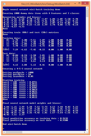
A good way to see where this article is headed is to examine the screenshot of a demo program shown in Figure 1. The demo program begins by generating 1,000 synthetic data items. Each data item has four input values and three output values. For example, one of the synthetic data items is:
-1.78 2.00 -7.51 2.07 1 0 0
 [Click on image for larger view.]
Figure 1. Mini-Batch Back-Propagation Training in Action
[Click on image for larger view.]
Figure 1. Mini-Batch Back-Propagation Training in Action
This data might correspond to a problem where you're trying to predict the political party affiliation (Democrat, Republican, Other) of a person based on their education, debt, income and urban-ness. The four input values are all between -10.0 and +10.0 and correspond to predictor values that have been normalized so that values less than zero are smaller than average, and values greater than zero are greater than average. The three output values correspond to a variable that can take on one of three categorical values. Using 1-of-N encoding, Democrat is (1, 0, 0), Republican is (0, 1, 0), and Other is (0, 0, 1).
So, the synthetic data item represents a person who has lower-than-average education (-1.78), higher-than-average debt (2.00), much-lower-than-average income (-7.51), and lives in a more urban environment than average (2.07). The person is a Democrat (1, 0, 0).
After the 1,000 data items were generated, the demo program split the data randomly, into an 800-item training set and a 200-item test set. The training set is used to create the neural network model, and the test set is used to estimate the accuracy of the model.
After the data was split, the demo program instantiated a neural network with five hidden nodes. Therefore the network has (4 * 5) + 5 + (5 * 3) + 3 = 43 weights and biases. The number of hidden nodes is arbitrary and in realistic scenarios must be determined by trial and error.
Next, the demo set the values of the back-propagation parameters. The maximum number of training iterations, maxEpochs, was set to 1,000. The learning rate, learnRate, controls how fast training works and was set to 0.05. In back-propagation, the momentum rate is an optional parameter to increase the speed of training and was not used in the demo. The batch size, batchSize parameter was set to 50. This means the 800 training items are processed 50 at a time.
During training, the demo program calculated and displayed the mean squared error, every 100 epochs. In general the error decreased over time, but there were a few jumps in error. This is typical behavior when using mini-batch back-propagation. When training finished, the demo displayed the values of the 43 weights and biases found. These values, along with the number of hidden nodes, essentially define the neural network model.
The demo concluded by using the weights and bias values to calculate the predictive accuracy of the model on the training data (771 correct out of 800 = 96.38%) and on the test data (190 correct out of 200 = 95.00%). The resulting model could then be used to predict the political party of a new person.
This article assumes you have at least intermediate level developer skills and a basic understanding of neural networks but does not assume you are an expert using the back-propagation algorithm. The demo program is too long to present in its entirety here, but complete source code is available in the download that accompanies this article. All normal error-checking has been removed to keep the main ideas as clear as possible.
Understanding Mini-Batch Training
The key to back-propagation training are quantities called gradients. During training, the current neural network weight and bias values, along with the training data input values, determine the computed output values. The training data has known, correct target output values. The computed output values might be greater than or less than the target values.
It's possible to compute a gradient for each weight and bias. A gradient is just a number like -0.83. The sign of the gradient (positive or negative) tells you whether to increase or decrease the value of the associated weight or bias so that the computed output values will get closer to the target output values. The magnitude of the gradient gives you a hint about how much the weight or bias value should change.
Note: technically, the values I've just described as "gradients" are really "partial derivatives." The collection of all partial derivatives, one for each weight and bias, is the gradient. However, it's common to refer to an individual partial derivative as a gradient.
In high-level pseudo-code, batch back-propagation is:
loop maxEpochs times
  for-each data item
    compute a gradient for each weight and bias
    accumulate gradient
  end-for
  use accumulated gradients to update each weight and bias
end-loop
In high-level pseudo-code, stochastic back-propagation is:
loop maxEpochs times
  for-each data item
    compute gradients for each weight and bias
    use gradients to update each weight and bias
  end-for
end-loop
In batch training, an accumulated gradient for each weight and bias is computed using all training data items, and then weights and biases are updated. In stochastic training (also called online training), after the gradients are computed for a single training item, weights and biases are updated immediately. Put another way, in stochastic training, the accumulated gradient values of batch training are estimated using single-training data items.
Mini-batch training is a combination of batch and stochastic training. Instead of using all training data items to compute gradients (as in batch training) or using a single training item to compute gradients (as in stochastic training), mini-batch training uses a user-specified number of training items. In pseudo-code, mini-batch training is:
loop maxEpochs times
  loop until all data items used
    for-each batch of items
      compute a gradient for each weight and bias
      accumulate gradient
    end-batch
    use accumulated gradients to update each weight and bias
  end-loop all item
end-loop
In the demo program, there are 800 training items and the batch size is set to 50. So during training, the gradients for each weight and bias are computed by processing 50 training items, then weights and biases are updated. It takes 800/50 = 16 batches of training items to process all training items.
Implementing Mini-Batch Training
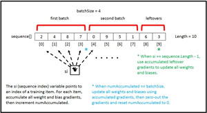
The diagram in Figure 2 shows how the demo program implements mini-batch training. In a simplified scenario, there are 10 training items which aren't shown. The batch size is set to 4. The array named sequence holds the indices of the 10 training items. The order of values in the array is random so that the training items will be processed in a random order.
 [Click on image for larger view.]
Figure 2. Implementing Mini-Batch Training
[Click on image for larger view.]
Figure 2. Implementing Mini-Batch Training
Variable si (sequence index) iterates through the sequence array. The value in the sequence array indicates which training data item to use. The training input values are fed to the neural network, output values are computed and compared to the target values. Then gradients are computed for each weight and bias, and accumulated.
When the number of processed training items, which is stored in variable numAccumulated, reaches the batch size, all weights and biases are updated using the accumulated gradients, and numAccumulated is reset to 0.
When the sequence index variable value reaches the length of the training data (10 in Figure 2), if numAccumulated > 0 then there are leftover accumulated gradients, so weights and biases are updated a final time. An alternative is to ignore the leftover accumulated gradient values, which is a form of what's called input node dropout training.
Notice that by setting the batch size to 1, mini-batch training becomes stochastic training. By setting the batch size to the length of the training data, mini-batch training becomes regular batch training.
The Demo Program
To create the demo program, I launched Visual Studio, selected the C# console application program template, and named the project MiniBatch. The demo has no significant .NET Framework version dependencies so any relatively recent version of VS should work. After the template code loaded, in the Solution Explorer window I renamed file Program.cs to MiniBatchProgram.cs and allowed VS to automatically rename class Program.
The overall structure of the demo program, with a few minor edits to save space, is presented in Listing 1. I removed unneeded using statements that were generated by the Visual Studio console application template, leaving just the one reference to the top level System namespace.
Listing 1: Demo Program Structure
using System;
namespace MiniBatch
{
  class MiniBatchProgram
  {
    static void Main(string[] args)
    {
      Console.WriteLine("Begin mini-batch demo");

      // All program calling statements here

      Console.WriteLine("End mini-batch demo");
      Console.ReadLine();
    }

    public static void ShowMatrix(double[][] matrix,
      int numRows, int decimals, bool indices) { . . }

    public static void ShowVector(double[] vector,
      int decimals, int lineLen, bool newLine) { . . }

    static double[][] MakeAllData(int numInput,
      int numHidden, int numOutput, int numRows,
      int seed) { . . }

    static void Split(double[][] allData, double trainPct,
      int seed, out double[][] trainData,
      out double[][] testData) { . . }

  } // Program class

  public class NeuralNetwork
  {
    private int numInput;
    private int numHidden;
    private int numOutput;

    private double[] inputs;
    private double[][] ihWeights;
    private double[] hBiases;
    private double[] hOutputs;

    private double[][] hoWeights;
    private double[] oBiases;
    private double[] outputs;

    private Random rnd;

    public NeuralNetwork(int numInput, int numHidden,
      int numOutput) { . . }

    private static double[][] Matrix(int rows,
      int cols, double v) { . . }

    private void InitializeWeights() { . . }

    public void SetWeights(double[] wts) { . . }

    public double[] GetWeights() { . . }

    public double[] ComputeOutputs(double[] xVals) { . . }

    private static double HyperTan(double x) { . . }

    private static double[] Softmax(double[] oSums) { . . }

    public double[] Train(double[][] trainData,
      int maxEpochs, int batchSize,
      double learnRate) { . . }

    private void ZeroOut(double[] vector) { . . }

    private void ZeroOut(double[][] matrix) { . . }

    private void Shuffle(int[] sequence) { . . }

    public double Error(double[][] trainData) { . . }

    public double Accuracy(double[][] testData) { . . }

    private static int MaxIndex(double[] vector) { . . }

  } // NeuralNetwork class
} // ns
All the control logic is in the Main method and all the classification logic is in a program-defined NeuralNetwork class. Helper method MakeAllData generates a synthetic data set. Method Split splits the synthetic data into training and test sets. Methods ShowData and ShowVector are used to display training and test data, and neural network weights.
The Main method (with a few WriteLine statements removed) begins by preparing to create the synthetic data:
static void Main(string[] args)
{
  Console.WriteLine("Begin mini-batch demo");
  int numInput = 4; // number features
  int numHidden = 5;
  int numOutput = 3; // number of classes for Y
  int numRows = 1000;
  int seed = 2; // gives representative demo
...
Next, the synthetic data is created:
Console.WriteLine("Generating " + numRows +
  " artificial data items with " + numInput + " features");
double[][] allData = MakeAllData(numInput, numHidden,
  numOutput, numRows, seed);
Console.WriteLine("Done");
To create the 1,000-item synthetic data set, helper method MakeAllData creates a local neural network with random weights and bias values. Then, random input values are generated, the output is computed by the local neural network using the random weights and bias values, and then output is converted to 1-of-N format.
Next, the demo program splits the synthetic data into training and test sets using these statements:
Console.WriteLine("Creating train and test matrices");
double[][] trainData;
double[][] testData;
SplitTrainTest(allData, 0.80, seed,
  out trainData, out testData);
Console.WriteLine("Done");
Console.WriteLine("Training data:");
ShowMatrix(trainData, 4, 2, true);
Console.WriteLine("Test data:");
ShowMatrix(testData, 4, 2, true);
Next, the neural network is instantiated like so:
Console.WriteLine("Creating a " +  numInput + "-" +
  numHidden + "-" + numOutput + " neural network");
NeuralNetwork nn = new NeuralNetwork(numInput,
  numHidden, numOutput);
The neural network has four inputs (one for each feature) and three outputs (because the Y variable can be one of three categorical values. The choice of five hidden processing units for the neural network is the same as the number of hidden units used to generate the synthetic data, but finding a good number of hidden units in a realistic scenario requires trial and error. Next, the mini-batch back-propagation parameter values are assigned with these statements:
int maxEpochs = 1000;
double learnRate = 0.05;
Console.WriteLine("Setting maxEpochs = " +
  maxEpochs);
Console.WriteLine("Setting batchSize = " +
  batchSize);
Console.WriteLine("Setting learnRate = " +
  learnRate.ToString("F2"));
Determining when to stop neural network training is a difficult problem. Here, using 1,000 iterations was arbitrary. The learning rate controls how much each weight and bias value can change in each update step. Larger values increase the speed of training at the risk of overshooting optimal weight values.
When training a neural network with back-propagation, it's common to use an optional technique called momentum. The demo program doesn't use momentum in order to keep the main ideas of mini-batch training as clear as possible. Using momentum helps prevents training from getting stuck with local, non-optimal weight values and also prevents oscillation where training never converges to stable values.
Training using mini-batch back-propagation is accomplished with these statements:
Console.WriteLine("Starting training");
double[] weights = nn.Train(trainData, maxEpochs,
  batchSize, learnRate);
Console.WriteLine("Done");
Console.WriteLine("Final weights and biases: ");
ShowVector(weights, 2, 10, true);
All the mini-batch logic is contained in method Train. The Train method stores the best weights and bias values found internally in the NeuralNetwork object, and also returns those values, serialized into a single result array. In a production environment you would likely save the model weights and bias values to a text file so they could be retrieved later, if necessary.
The demo program concludes by calculating the prediction accuracy of the neural network model:
...
  double trainAcc = nn.Accuracy(trainData);
  Console.WriteLine("Final accuracy on train data = " +
    trainAcc.ToString("F4"));
  double testAcc = nn.Accuracy(testData);
  Console.WriteLine("Final accuracy on test data = " +
    testAcc.ToString("F4"));
  Console.WriteLine("End back-propagation demo");
  Console.ReadLine();
} // Main
The accuracy of the model on the test data gives you a very rough estimate of how accurate the model will be when presented with new data that has unknown output values. The accuracy of the model on the training data is useful to determine if model over-fitting has occurred. If the prediction accuracy of the model on the training data is significantly greater than the accuracy on the test data, then there's a strong likelihood that over-fitting has occurred and re-training with new parameter values is necessary.
The Training Method
The code for the training method is presented in Listing 2. Inside the main processing loop, helper method Shuffle uses the Fisher-Yate mini-algorithm to scramble the order of the training item indices stored in the sequence array. When using stochastic or mini-batch training it's important to visit training data in a random order. When using full batch training the order of the training data doesn't matter because all training items are used to compute the gradients.
Listing 2: The Training Method
public double[] Train(double[][] trainData, int maxEpochs,
  int batchSize, double learnRate)
{
  double[][] hoGrads = Matrix(numHidden, numOutput, 0.0);
  double[] obGrads = new double[numOutput];
  double[][] ihGrads = Matrix(numInput, numHidden, 0.0);
  double[] hbGrads = new double[numHidden];
  double[] oSignals = new double[numOutput];
  double[] hSignals = new double[numHidden];

  int epoch = 0;
  double[] xValues = new double[numInput]; // inputs
  double[] tValues = new double[numOutput]; // targets
  double derivative = 0.0;
  double errorSignal = 0.0;

  int[] sequence = new int[trainData.Length];
  for (int i = 0; i < sequence.Length; ++i)
    sequence[i] = i;

  int errInterval = maxEpochs / 10; // to check error

  while (epoch < maxEpochs) // main training loop
  {
    ++epoch;

    if (epoch % errInterval == 0 && epoch < maxEpochs)
      // Compute and display curr error

    Shuffle(sequence); // visit in random order
    int ti = 0; // index into training data row
    int numAcc = 0; // number accumulated gradients

    for (int si = 0; si < sequence.Length; ++si)
    {
      ti = sequence[si]; // training item to process
      Array.Copy(trainData[ti], xValues, numInput);
      Array.Copy(trainData[ti], numInput,
        tValues, 0, numOutput);
      ComputeOutputs(xValues);

      // 1. Compute output node signals
      // 2. Compute and accumulate hidden-to-output
      //    weight gradients using output signals
      // 3. Compute hidden node signals
      // 4. Compute and accumulate input-hidden
            weight gradients
      // 5. Compute and accumulate hidden node
             bias gradients

      ++numAcc; // processed an item

      if (numAcc == batchSize ||
        (si == trainData.Length - 1 && numAcc > 0) ||
          numAcc == trainData.Length)
      {
        // A. Update input-to-hidden weights
        // B. Update hidden biases
        // C. Update hidden-to-output weights
        // D. Update output node biases

        // Zero-out accumulated gradients
        ZeroOut(ihGrads);
        ZeroOut(hbGrads);
        ZeroOut(hoGrads);
        ZeroOut(obGrads);

        numAcc = 0; // reset number accumulated

      } // End we-have-a-batch
    } // End each sequence index
  } // Each epoch

  double[] bestWts = GetWeights();
  return bestWts;

} // Train
The if-condition to check if it's time to update the neural network weights and biases has three conditions. The first condition, (numAcc == batchSize), is the usual case when a batch of training items has been processed. The second condition, (si == trainData.Length - 1 && numAcc > 0), occurs when there are leftover, unprocessed gradients. The third condition, (numAcc == trainData.Length), catches the case when the batch size has been set to the number of training items, which is equivalent to full batch training.
Wrapping Up
So, which form of neural network training is best -- batch, stochastic/online or mini-batch? In my opinion research results are inclusive and suggest that the best approach to use depends on your particular problem. As a general rule of thumb, mini-batch training works very well when you have a large neural network or the training set has lots of redundant data.
A disadvantage of mini-batch training compared to stochastic and batch training is that you must specify the batch size in addition to values for the number of hidden nodes, the learning rate, the momentum rate, and the maximum number of training epochs. The batch size, like the other free parameters, must be determined by trial and error.