Because there are three hidden nodes, there are three context nodes, and because every context node is connected to each hidden node, there are 3 * 3 = 9 context-to-hidden node weights. The context-to-hidden node weights are set to chWt[0][0] = 0.18, chWt[0][1] = 0.19, chWt[0][2] = 0.20, chWt[1][0] = 0.21, chWt[1][1] = 0.22, chWt[1][2] = 0.23, chWt[2][0] = 0.24, chWt[2][1] = 0.25, chWt[2][2] = 0.26. Not all of the context-to-hidden weight values are explicitly labeled in Figure 2 because there wasn't enough space.

First, the preliminary sum for hidden node 0 is calculated as hSum[0] = (1.0)(0.01) + (2.0)(0.04) + (0.30)(0.18) + (0.40)(0.21) + (0.50)(0.24) + 0.07 = 0.4180. Notice the preliminary sum for a recurrent network hidden node is calculated just like the preliminary sum for a regular network except that the values of the context nodes act as additional input values.

In the same way, hSum[1] = (1.0)(0.02) + (2.0)(0.05) + (0.30)(0.19) + (0.40)(0.22) + (0.50)(0.25) + 0.08 = 0.4700. And hSum[2] = (1.0)(0.03) + (2.0)(0.06) + (0.30)(0.20) + (0.40)(0.23) + (0.50)(0.26) + 0.09 = 0.5220.

Next, the tanh activation function is applied to each of the preliminary sums to give the values of the hidden nodes. So, hNode[0] = tanh(0.4180) = 0.3952, hNode[1] = tanh(0.4700) = 0.4382, and hNode[2] = tanh(0.5220) = 0.4792.

Next, the output node preliminary sums are calculated. For output node 0, oSum[0] = (0.3952)(0.10) + (0.4382)(0.12) + (0.4792)(0.14) + 0.16 = 0.3192. In the same way, oSum[1] = (0.3952)(0.11) + (0.4382)(0.13) + (0.4792)(0.15) + 0.17 = 0.3423.

The final output node values are calculated by applying the softmax activation function. So output[0] = exp(0.3192) / (exp(0.3192) + exp(0.3423)) = 1.3760 / 2.7842 = 0.4942, and output[1] = exp(0.3423) / (exp(0.3192) + exp(0.3423)) = 1.4082 / 2.7842 = 0.5058, as shown in Figure 2.

The last step for a recurrent neural network is to copy the values of the hidden nodes to the context nodes. So, cNode[0] = hNode[0] = 0.3952, cNode[1] = hNode[1] = 0.4382 and cNode[2] = hNode[2] = 0.4792. These context node values will act as supplementary inputs for the next set of input data values.

The essence of a recurrent neural network is that hidden node values are saved and used with the next set of input values. Put another way, the output values of a recurrent neural network depend on the current input values and the hidden node values derived from the previous set of input values. This means the network maintains partial state.

By maintaining state, recurrent neural networks can predict values that depend in some way on previous input values. For example, recurrent neural networks work very well with handwriting recognition because the value of a letter in a word depends to some extent on the value of the previous letter in the word.

A Demo Program
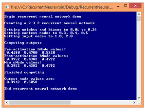
Figure 3 shows a demo of a recurrent neural network. The demo program corresponds to the network in Figure 2. The demo begins by creating a 2-3-2 recurrent neural network. Next, the weights and biases are set to 0.01 through 0.26. Because there are two input and three hidden nodes, there are 2 * 3 = 6 input-to-hidden weights that are set to 0.01 through 0.06.

The three hidden node biases are set to 0.07, 0.08 and 0.09. The 3 * 2 = 6 hidden-to-output weights are set to 0.10 through 0.15. The two output node biases are set to 0.16 and 0.17. The 3 * 3 = 9 context-to-hidden weights are set to 0.18 through 0.26. In a non-demo scenario, weights and biases are usually initialized to small random values.

Next, the demo sets the initial values of the three context nodes to 0.3, 0.4 and 0.5. These values are arbitrary. In a non-demo scenario, initial context node values often depend on the particular problem scenario. In many situations the initial context node values are set to 0.0 or 0.5.

The demo sets the input node values to 1.0 and 2.0 and then feeds those values to the recurrent network. The demo displays the pre-activation and post-activation values of the hidden nodes, and the new values of the context nodes. Notice the new context node values are copies of the post-activation hidden node values. The demo concludes by displaying the computed output values (0.4942, 0.5058).

The demo program is too long to present in its entirety here, but complete source code is available in the download that accompanies this article. All normal error checking has been removed to keep the main ideas of neural network models as clear as possible.

The Demo Program Structure
To create the demo program I launched Visual Studio and selected the C# console application project template. I named the project RecurrentNeural. The demo has no significant Microsoft .NET Framework dependencies, so any version of Visual Studio will work.

After the template code loaded, in the Solution Explorer window I right-clicked on file Program.cs and renamed it to the more descriptive RecurrentNeuralProgram.cs and then allowed Visual Studio to automatically rename class Program. At the top of the template generated code in the Editor window, I deleted all unnecessary using statements, leaving just the reference to the top-level System namespace.

The overall structure of the demo program is shown in Listing 1. All of the program control logic is in the Main method. All of the recurrent neural network logic is contained in a program-defined RecurrentNetwork class.

using System;
using System.IO;
namespace NeuralModels
{
  class NeuralModelsProgram
  {
    static void Main(string[] args)
    {
      // All program control statements
    }
   
    public static void ShowMatrix(double[][] matrix,
      int numRows, int decimals,
      bool indices) { . . }
    
    public static void ShowVector(double[] vector,
      int decimals, int lineLen,
      bool newLine) { . . }
  }

  public class RecurrentNetwork { . . }

} // ns

The Main method creates the network with these statements:

int numInput = 2;
int numHidden = 3;
int numOutput = 2;
int seed = 0;
RecurrentNetwork rn =
  new RecurrentNetwork (numInput, numHidden, numOutput, seed);

The seed value is used to instantiate a Random object that's used to initialize weights and biases to random values. In a non-demo scenario, neural networks often use a Random object to shuffle the order of training data items and to split data into training and test sets.

The weights and biases are set with these statements:

double[] wts = new double[] { 0.01, 0.02, 0.03, 0.04, 0.05, 0.06,
  0.07, 0.08, 0.09,
  0.10, 0.11, 0.12, 0.13, 0.14, 0.15,
  0.16, 0.17,
  0.18, 0.19, 0.20, 0.21, 0.22, 0.23, 0.24, 0.25, 0.26 };
Console.WriteLine("Setting weights and biases to 0.01 to 0.26");
rn.SetWeights(wts);

The initial values of the context nodes are set with these statements:

double[] cValues = new double[] { 0.3, 0.4, 0.5 };
Console.WriteLine("Setting context nodes to 0.3, 0.4, 0.5");
rn.SetContext(cValues);

In most non-demo scenarios you probably wouldn't need a SetContext method because the initial values of the context nodes would likely be set in the class constructor.

The input values are set and output values are computed like so:

double[] xValues = new double[] { 1.0, 2.0 };
Console.WriteLine("Setting input nodes to 1.0, 2.0");

double[] yValues = rn.ComputeOutputs(xValues);

Console.WriteLine("Output node values are:");
ShowVector(yValues, 4, yValues.Length, true);

The values of the hidden and context nodes are displayed by WriteLine statements in method ComputeOutputs. In most situations you wouldn't display these values, or perhaps you'd modify ComputeOutputs with a Boolean parameter named something like verbose to control whether to display the values.

The RecurrentNetwork Class
The structure of the RecurrentNetwork class is presented in Listing 2.

public class RecurrentNetwork
{
  private int numInput; // Number input nodes
  private int numHidden;
  private int numOutput;
  
  private double[] inputs;
  private double[][] ihWeights; // Input-hidden
  private double[] hBiases;
  private double[] hNodes; // Hidden nodes
  private double[][] chWeights; // Context-hidden
  private double[] cNodes; // Context nodes
  private double[][] hoWeights; // Hidden-output
  private double[] oBiases;
  private double[] outputs;
  private Random rnd;

  public RecurrentNetwork(int numInput, int numHidden,
    int numOutput, int seed) { . . }
  private static double[][] MakeMatrix(int rows,
    int cols) { . . }
  private void InitializeWeights() { . . }
  private void InitializeContext() { . . }
  public void SetWeights(double[] weights) { . . }
  public double[] GetWeights() { . . }
  public void SetContext(double[] values) { . . }
  public double[] ComputeOutputs(double[] xValues) { . . }
  private static double HyperTan(double x) { . . }
  private static double[] Softmax(double[] oSums) { . . }
}

Compared to a regular feed-forward neural network, a recurrent network has two additional fields. Array cNodes holds the values of the context nodes. Array-of-arrays style matrix chWeights holds the values of the context-to-hidden node weights. Notice there's no need for a field named numContext to hold the number of context nodes because in a simple recurrent network the number of context nodes is equal to the number of hidden nodes.

The definition of method ComputeOutputs begins as:

public double[] ComputeOutputs(double[] xValues)
{
  double[] hSums = new double[numHidden];
  double[] oSums = new double[numOutput];
... 

Arrays hSums and oSums hold the preliminary, pre-activation values of the hidden nodes and the output nodes. Note that in C#, instantiating an array initializes all cell values to 0.0, so explicit initialization isn't necessary. Next, input values from the xValues parameter array are copied into the input nodes:

for (int i = 0; i < xValues.Length; ++i)
  this.inputs[i] = xValues[i];

No error checking is performed, which keeps the size of the code smaller. Next, the preliminary hidden node sums are calculated as described previously:

for (int j = 0; j < numHidden; ++j) 
  for (int i = 0; i < numInput; ++i)
    hSums[j] += this.inputs[i] * this.ihWeights[i][j];

Next, the contribution of the context nodes is added to the hidden nodes preliminary sums:

for (int j = 0; j < numHidden; ++j)
  for (int c = 0; c < numHidden; ++c)
    hSums[j] += this.cNodes[c] * chWeights[c][j];

I've deliberately been inconsistent with regard to the use of an explicit "this" qualifier for class members in order to point out that this isn't very good practice. Next, the hidden node biases are added:

for (int j = 0; j < numHidden; ++j)
  hSums[j] += this.hBiases[j];

Many neural network implementations treat biases as special weights associated with a dummy input that has a constant 1.0 value. This practice started because it makes equations in mathematical proofs easier to work with, but from an engineering point of view it makes code harder to read and more error-prone, in my opinion. Next, the hidden node activation function is applied:

for (int j = 0; j < numHidden; ++j) 
  this.hNodes[j] = HyperTan(hSums[j]);

The demo uses a hardcoded hyperbolic tangent function rather than passing in the function to use as a parameter. Writing custom neural network code for your own use allows you to be very efficient, as opposed to writing code for use by others through an API set. Next, the output node preliminary sums are computed:

for (int k = 0; k < numOutput; ++k) 
  for (int j = 0; j < numHidden; ++j)
    oSums[k] += hNodes[j] * hoWeights[j][k];

Notice that in this variation of recurrent neural networks, the context nodes do not directly contribute to the output values. There are many types of recurrent networks. For example, in one variation called Jordan networks, the context nodes are fed from the output nodes instead of the hidden nodes. Next, the output node bias values are added and then the softmax activation function is applied:

for (int k = 0; k < numOutput; ++k) 
  oSums[k] += oBiases[k];

double[] softOut = Softmax(oSums); 
for (int k = 0; k < numOutput; ++k)
  outputs[k] = softOut[k];

Unlike the hidden layer activation function that works on a single node, the softmax function works on all output nodes together because all their values are needed. Next, the values of the hidden nodes are copied into the context nodes:

for (int j = 0; j < numHidden; ++j)
  cNodes[j] = hNodes[j];

When the next input values arrive, the context nodes now have some memory of the previous state of the network. Method ComputeOutputs concludes by copying the values in the output nodes to an explicit return value so they can be easily accessed by the calling code:

...
  double[] retResult = new double[numOutput];
  for (int k = 0; k < numOutput; ++k)
    retResult[k] = outputs[k];
  return retResult;
} // ComputeOutputs

A common design alternative, but one I don't like too much, is to code ComputeOutputs so that it returns void and implement a utility method or property named something along the lines of GetOutputs that returns the values in the output nodes.

Wrapping Up
The code and explanation presented in this article should get you up and running if you want to experiment with simple recurrent neural networks. The architecture described here, with a single set of context nodes, maintains partial state. A way to extend the idea is to use multiple layers of context nodes. For example, you could use three layers of context nodes where the first layer would hold the values of the hidden nodes associated with the previous set of inputs. The second layer would hold hidden node values associated with the inputs before the previous inputs. The third layer would hold hidden node values associated with inputs that occurred three sets before the current inputs.

Training a recurrent neural network isn't easy. There are many (roughly a dozen) different variations of the standard back-propagation algorithm that can be used. The fact that there are so many different training techniques suggests that all of them have weaknesses. A promising training approach for recurrent neural networks that, to the best of my knowledge hasn't been thoroughly investigated, is to use a swarm-based technique such as simplex optimization or particle swarm optimization.