The Data Science Lab
How the R Language Does OOP
It's not quite like C# or Python, but the R language's object-oriented programming capabilities are getting better with each iteration. Let's take a look at what .NET developers are able do now with OOP in R6.
The R language was created primarily to perform statistical analyses in an interactive environment using hundreds of built-in functions such as t.test for Welch's t-test and aov for analysis of variance. From the very beginning R has had a basic scripting language with loop control structures, if...then decision control, and so on, but until recently, R object-oriented programming (OOP) capabilities were somewhat limited compared to languages such as C# and Python.
About 18 months ago, OOP with R took a significant step forward with the release of the R6 package. In this article I'll give you a quick tour of OOP with R6. Although the documentation for R6 is quite good, it's very detailed, which obscures some of the main ideas, and it assumes you're an experienced R user. I'll explain programming with R6 (technically scripting because R is interpreted rather than compiled) from the point of view of a .NET developer who is new to R.
To get an idea of where this article is headed, take a look at the screenshot of a demo R session in Figure 1. The outer container window is the Rgui.exe shell. Inside the shell, the window on the left is the R Console where you can issue interactive commands. Here, I use the setwd function to set the working directory to the location of my demo R files, then I use the source function to execute the TestPerson.R file.
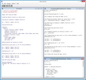 [Click on image for larger view.]
Figure 1. OOP with R6 Demo Session
[Click on image for larger view.]
Figure 1. OOP with R6 Demo Session
The upper-right window inside the shell is the source R code for the TestPerson.R script. That script uses a R6 class that defines a Person object. In most realistic scenarios an R6 class would contain numeric arrays and matrices, but a Person class is easy to understand and is a common "Hello World" example for OOP. The source code for the Person class is partially shown in the lower-right window.
In Figure 1, notice that there's a warning message displayed in the console after the demo script finishes execution because I wrote the demo code using R version 3.1.2 (a slightly older version released in 2015), but the R6 code was written with R version 3.1.3. Because R is open source and has many authors, and different packages have different dependencies, maintaining R package compatibility can be mildly annoying at times. Some R users and programmers sometimes call this situation "package hell."
Installing R and R6
If you don't have R on your system, installing R (and uninstalling) is very easy. Do an Internet search for "Install R" and you'll find a page on the cran.r-project.org Web site with a link labeled, "Download R 3.2.x for Windows." Click that link and you'll get an option to run a self-extracting installer file named something like R-3.2.x-win.exe. Click on the Run button presented to you by your browser to launch the installer. You can accept all the configuration defaults and installation is quick.
To launch the Rgui program, open a file explorer and navigate to the C:\Program Files\R\R-3.2.x\bin\x64 directory. To launch Rgui in standard mode, double-click on file Rgui.exe and the Rgui shell with an R Console window will launch. However, you might need administrator privileges to install packages, so I suggest right-clicking on Rgui.exe and selecting the "Run as administrator" option from the context menu. After the shell launches, you can clear the start messages with Ctrl+L.
The base R language does not include the R6 package. R has hundreds of available packages written by the R open source community. You can display a list of all the packages that are currently installed on your machine by typing the command:
> installed.packages()
To install the R6 package, make sure you're connected to the Internet, then type the command:
> install.package("R6")
This will launch a tall, thin window that lists approximately 130 mirror sites that might contain the R6 package. Click on a mirror site. If that mirror site is up and running, and has the R6 package, R6 will be installed on your system quickly and you'll see a success message that reads, "package R6 successfully unpacked and MD5 sums checked. The downloaded binary packages are in C:\xxx."
If the R6 installation fails because the mirror site you selected was down, you can try a different mirror site by typing the command:
> chooseCRANmirror(graphics=getOption("menu.graphics"))
To remove an R package you can type a command like:
> remove.packages("R6")
Package removal, like installation, is quick and easy.
The Class Definition Code
When learning about OOP in a new programming language, there's always a chicken-and-egg issue: do you look at the class definition first and then see how the class is used to create an object, or do you look at the calling code first and then examine the class definition code? I'll present the class definition first.
To create the class definition script, on the Rgui menu bar I clicked File | New Script. This gave me an editor window. I clicked File | Save As and saved the (currently empty) script as PersonClass.R in C:\OopUsingR6 on my machine.
The complete code for file PersonClass.R is presented in Listing 1. The first three lines of code are:
# file: PersonClass.R
# R 3.1.2
library(R6)
After commenting the name of the script, I place a comment that indicates which version of R I'm using. Notice that my version of R is slightly out of date. Next, the library function is used to load the R6 package. You can think of this as somewhat similar to adding a reference to a .NET DLL assembly to a C# program. Instead of using the library function, I could've used the require function.
Listing 1: Class Definition Code
# file: PersonClass.R
# R 3.1.2

library(R6)

Person <- R6Class("Person",

  private = list(
    last.name = NULL,
    first.name = NULL,
    pay.rate = NULL
  ), # private

  public = list(
    initialize = function(last.name, first.name, pay.rate) {
      private$last.name <- last.name
      private$first.name <- first.name
      private$pay.rate <- pay.rate
    },

    setRate = function(rate) {
      private$pay.rate <- rate
    },

    getRate = function() {
      return(private$pay.rate)
    },

    display = function() {
      cat("[", private$last.name, ", " ,
          private$first.name, ", $" ,
          formatC(private$pay.rate, digits=2, format="f") ,
          "]\n", sep="")
    }
  ) # public

) # Person
The structure of the class definition is:
Person <- R6Class("Person",
  private = list(
    # private variables and functions here
  ),
  public = list(
    # public variables and functions here
  )
}
If you're a C# programmer, the syntax might look a bit unusual, but should make sense. Instead of declaring member fields and methods with public and private scope qualifiers, in R6 you have a list collection of private items and a list collection of public items. This somewhat resembles C++ class definitions that have private and public code areas.
Notice that the class definition has two names: Person with and without quotes. Although the two names don't have to match, there's no reason to make them different.
The private variables are:
private = list(
  last.name = NULL,
  first.name = NULL,
  pay.rate = NULL
),
In R, it's common to use the '.' character in variable names to make them more readable. I prefer using an underscore (last_name) or camel casing (lastName) but use the '.' here to illustrate the idea.
The public class constructor is:
initialize = function(last.name, first.name, pay.rate) {
  private$last.name <- last.name
  private$first.name <- first.name
  private$pay.rate <- pay.rate
},
In R6, the initialize function is used to instantiate an object. Here, the parameter names are the same as the field variable names. This is OK because private and public class variables are accessed by prepending the "private" or "self" keywords, respectively. Alternatively, I could've written code like:
initialize = function(ln, fn, pr) {
  private$last.name <- ln
  private$first.name <- fn
  private$pay.rate <- pr
},
The class definition has two public methods to fetch and modify the pay.rate member variable:
setRate = function(rate) {
  private$pay.rate <- rate
},
getRate = function() {
  return(private$pay.rate)
},
These functions closely resemble their C# property method counterparts. I could've defined similar functions for the last.name and first.name variables.
The function names used here, setRate and getRate, aren't very good style because they don't quite match the corresponding class variable pay.rate name. A better naming approach -- in my opinion – would've been to call the member variable payRate and name the functions set_payRate and get_payRate, similar to the Java naming convention.
The last function defined in the Person class displays an object directly to the R Console:
display = function() {
  cat("[", private$last.name, ", " ,
    private$first.name, ", $" ,
    formatC(private$pay.rate, digits=2, format="f") ,
    "]\n", sep="")
}
Calling this function produces output like:
[Smith, James, $19.00]
In C# the usual approach would be to define a ToString method for the object and then call like:
Console.WriteLine(p1.ToString());
You could take this approach with R, too, but in R displaying directly to the console is more common.
The Demo Script
To create the test script, on the Rgui menu bar I clicked File | New Script. This gave me an editor window. I clicked File | Save As and saved the (empty) script as TestPerson.R in a C:\OopUsingR6 directory (the same location as the PersonClass.R file).
The first four lines of the test script are:
# file: TestPerson.R
# R 3.1.2
source("PersonClass.R") # load
cat("\nBegin OOP using R6 demo \n\n")
The source function is used to load into memory the file that contains the code that defines the Person class. Because there's no path to the file name, it's assumed that the file is located in the same directory as the test harness script. The cat function displays a start message.
Next, the test script instantiates a Person object:
cat("Creating Person object p1 using new() \n\n")
p1 <- Person$new("Smith", "James", 19.00)
This creates a Person object named p1 with a last name of "Smith" and a first name of "James" and a pay rate of $19.00. The key idea here is that you use the new function appended to a class name with the '$' character to instantiate an R6 object by calling the class initialize function. In C#, this would look like:
Person p1 = new Person("Smith", "James", 19.00);
The R6 design and calling syntax should feel familiar to you. In this example, it's clear that "Smith" is almost certainly the last name and "James" is the first name, but because R supports named-parameter calls, for improved readability at the expense of wordiness you can write code like:
p1 <- Person$new(last.name="Smith",
                 first.name="James",
                 pay.rate=19.00)
Next, the demo script displays the newly created Person object:
cat("Calling p1.display() member function \n\n")
cat("p1 : ")
p1$display()
The Person class definition contains a program-defined member function display that prints directly to the R Console. The output is:
Calling p1.display() member function
p1 : [Smith, James, $19.00]
Next, the demo prints the Person object in a different way:
cat("\nCalling print(p1)\n\n")
print(p1)
Here, the R built-in print function is used instead of the class member function. The output is:
<Person>
  Public:
    clone: function (deep = FALSE)
    display: function ()
    getRate: function ()
    initialize: function (last.name, first.name, pay.rate)
    setRate: function (rate)
  Private:
    first.name: James
    last.name: Smith
    pay.rate: 19
Notice that there's an extra clone function listed. I'll explain in a moment. In general, you'll use a custom display function in program-defined scripts, and use the built-in print function interactively to examine objects.
Next, the test script illustrates the use of the clone function:
cat("\nMaking person p2 using p1.clone() \n")
p2 <- p1$clone()

cat("\nModifying p2 pay.rate to 22.00 using setRate() \n\n")
p2$setRate(22.00)

cat("p2 : "); p2$display()
cat("p1 : "); p1$display()
The output is:
Making person p2 using p1.clone()

Modifying p2 pay.rate to 22.00 using setRate()

p2 : [Smith, James, $22.00]
p1 : [Smith, James, $19.00]
The point here is that when you define an R6 class, you automatically get a clone function. When you call clone, you get a value copy rather than a reference copy. In other words, the cloned object is separate from the original object. Notice that the change to the Person p2 pay.rate has no effect on the p1 pay.rate variable.
Next, the demo illustrates how to make a reference copy:
cat("\nAssigning p3 <- p1 \n\n")
p3 <- p1

cat("Modifying p3 pay.rate to 30.00 using setRate() \n\n")
p3$setRate(30.00)

cat("p3 : "); p3$display()
cat("p1 : "); p1$display()
The output is:
Assigning p3 <- p1

Modifying p3 pay.rate to 30.00 using setRate()

p3 : [Smith, James, $30.00]
p1 : [Smith, James, $30.00]
Here, a change to the Person p3 pay.rate also affects the original p1 pay.rate. Both p3 and p1 point to the same object in memory so a change to one object affects the other object, too. To summarize, value copies and reference copies in R6 work in much the same way as they do in C# and you have to be careful to avoid accidentally creating any unwanted side effects.
The two demo scripts are organized with the class definition code and the calling code are in separate files. It would've been possible to place the class definition code directly inside the test script.
Wrapping Up
The explanation presented in this article should give you all the information you need to get up and running with R6 classes. R6 classes support some additional features. R6 classes support inheritance, but at least in my experience, this is rarely needed when programming with R. Other rarely used features of R6 classes include active bindings, non-portable classes, extending a class definition, deep cloning, and finalizers.
The base R language has three different built-in OOP models named S3, S4 and RC ("Reference Classes"). The S3 and S4 models are named as they are because they were created in the S language, which is the predecessor of R. At one point there was a project to create a more modern OOP model and it was named R5 (R for the language, 5 because the previous models were 3 and 4) but work on R5 was discontinued. RC classes are more sophisticated than S3 and S4 classes and R6 classes are essentially an improved version of RC classes.
I spoke with the author of the R6 package, Winston Chang. Winston considers the R6 package stable and he doesn't have any immediate plans for significant changes to R6. He said he may consider adding support for static variables and functions to R6 at some point in the future.