The Data Science Lab
Neural Networks Using the R nnet Package
The R language simplifies the creation of neural network classifiers with an add-on that lays all the groundwork.
A neural network classifier is a software system that predicts the value of a categorical value. For example, a neural network could be used to predict a person's political party affiliation (Democrat, Republican, Other) based on the person's age, sex and annual income.
There are many ways to create a neural network. You can code your own from scratch using a programming language such as C# or R. Or you can use a tool such as the open source Weka or Microsoft Azure Machine Learning. The R language has an add-on package named nnet that allows you to create a neural network classifier. In this article I'll walk you through the process of preparing data, creating a neural network, evaluating the accuracy of the model and making predictions using the nnet package.
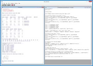
The best way to see where this article is headed is to take a look at the screenshot of a demo R session in Figure 1. All of the source code for the demo program is presented in this article. You can also get the complete demo program and the associated data file I used in the code download that accompanies this article.
 [Click on image for larger view.]
Figure 1. Neural Network Classification Using the nnet Package
[Click on image for larger view.]
Figure 1. Neural Network Classification Using the nnet Package
In the R Console window, I started my session by entering three commands:
> rm(list=ls())
> setwd("C:\\NnetDemo")
> source("neuralDemo.R")
The first command removes all existing objects from the current workspace so I can start with a clean memory set. The second command specifies the working directory so that I won't need to fully qualify the path to my R program (technically a script because R is interpreted) and to my source data file. The third command executes my demo program, which is named neuralDemo.R.
The goal of the program is to predict species of iris flower ("setosa," "versicolor," virginica") from four input values: the sepal length and width, and the petal length and width. A sepal is a green leaf-like structure. This problem is the Hello World example for neural network classification.
The first part of the program output in the Console shell shows six lines of the 150-line raw data file:
Sepal.length  Sepal.width  Petal.length  Petal.width  Species
1       5.1     3.5          1.4           0.2         I. setosa
2       4.9     3            1.4           0.2         I. setosa
...
51      7       3.2          4.7           1.4         I. versicolor
52      6.4     3.2          4.5           1.5         I. versicolor
...
101     6.3     3.3          6             2.5         I. virginica
102     5.8     2.7          5.1           1.9         I. virginica
The next part of the output shows six lines of the data that has been processed so that it can be used by the functions in the nnet package:
       SepLen  SepWid  PetLen  PetWid  Species
1       5.1     3.5     1.4     0.2     s
2       4.9     3       1.4     0.2     s
...
51      7       3.2     4.7     1.4     c
52      6.4     3.2     4.5     1.5     c
...
101     6.3     3.3     6       2.5     v
102     5.8     2.7     5.1     1.9     v
The next part of the program output displays 30 random indices that define which of the 150 data items will be used to train the neural network:
The training sample indices are:
 [1]  14  19  28  43  10  41  42  29  27   3  61  59  83  69  86  73  82
[18]  93  66  94 147 111 132 106 113 118 101 117 137 114
The next part of the program output shows progress messages that are generated automatically while the neural network is being created and trained:
Creating and training a neural network . .
# weights:  19
initial  value 36.853825
iter  10 value 14.548021
iter  20 value 13.863357
iter  30 value 5.523727
iter  40 value 0.031016
iter  50 value 0.022324
final  value 0.022324
stopped after 50 iterations
The last part of the program output displays a confusion matrix, which is an indication of the accuracy of the trained neural network model:
Confusion matrix for resulting nn model is:
     c  s  v
  c 36  0  4
  s  0 40  0
  v  2  0 38
There are a total of 150 data items. The program used 30 randomly selected data items to train the neural network. The confusion matrix was created using the 120 data items that weren't used for training. The value of 36 in the upper-left-hand corner indicates that 36 of the data items, which are species versicolor, were correctly predicted as versicolor. The number 4 in the top row indicates that there were 4 data items that are species versicolor, but were incorrectly predicted to be virginica.
The values on the diagonal of the confusion matrix are correct predictions on the holdout data, and the values off the diagonal are incorrect predictions. So the neural network model has an accuracy of 114 / 120 = 0.95. You can loosely interpret this to be the estimated accuracy that you'd get when using the neural network to predict the species of a new flower where the actual species isn't known.
The Demo Program
If you want to copy-paste and run the demo program, and you don't have R installed on your machine, installation (and just as important, uninstallation) is quick and easy. Do an Internet search for "install R" and you'll find a URL to a page that has a link to "Download R for Windows." I'm using R version 3.3.0, but by the time you read this article, the current version of R will likely have changed. If you click on the download link, you'll launch a self-extracting executable installer program. You can accept all the installation option defaults, and R will install in about 30 seconds. Just as important, installing R will not damage your system, and you can quickly and cleanly uninstall R using the Windows Control Panel, Programs and Features uninstall option.
To create the demo program, I navigated to directory C:\Program Files\R\R-3.3.0\bin\x64 and double-clicked on the Rgui.exe file. After the shell launched, from the menu bar I selected the File | New script option, which launched an untitled R Editor window. I added two comments to the script, indicating the file name and R version I'm using:
# neuralDemo.R
# R 3.3.0
Next, I did a File | Save as, to save the script. I put my demo script at C:\NnetDemo, but you can use any convenient directory.
Before adding code to the demo program, I created the raw source data file. You can find Fisher's Iris Data in several places on the Internet. I got the data from the Wikipedia entry. I copy-pasted the data, including the header line, into Notepad. I replaced the blank space field separators with commas because the Species values annoyingly contain spaces, for example "I. setosa," which is short for Iris setosa.
I saved the data as file IrisData.txt in the NnetDemo directory, but I could have put the file anywhere. The data file has 150 items, one per line. The first 50 lines are all setosa. The next 50 items on lines 51 to 100 are all versicolor. The last 50 items on lines 101 to 150 are all virginica.
After creating and saving the data, I went back to the Editor window in the RGui program. The demo program code begins by attaching the nnet package and loading the raw data into a data frame object:
library(nnet)
cat("\nBegin neural network using nnet demo \n\n")
cat("Original Fisher's Iris data: \n\n");
origdf <- read.table("IrisData.txt", header=TRUE, sep=",")
When you install R, you get 30 packages with names such as base and stats. You can see the 30 packages at C:\Program Files\ C:\Program Files\R\R-3.3.0\library. However, not all 30 packages are directly visible to you by default. The nnet package is one such package. To bring a package into scope you can use the library function or the nearly equivalent require function.
The demo program loads the raw data into an R data frame object named origdf using the read.table function. In R, the "." character can be used in identifier names so read.table is just a function name and doesn't mean something like the table method of the read object. Because the data file is in the same directory as the program file, I didn't need to add path information to the file name.
Next, the demo code displays parts of the data frame holding the raw data using the write.table function:
write.table(origdf[1:2, ], col.names=TRUE, sep="\t", quote=FALSE)
cat(". . . \n")
write.table(origdf[51:52, ], col.names=FALSE, sep="\t", quote=FALSE)
cat(". . . \n")
write.table(origdf[101:102, ], col.names=FALSE, sep="\t", quote=FALSE)
cat("\n")
I could've displayed all 150 lines with a single statement:
print(origdf)
Notice the comma in the indexing syntax, for example origdf[1:2, ], which means "rows 1 to 2 and all columns." The space following the embedded comma is just for clarity and could've been omitted.
Preparing the Data
The data frame now has the categorical data that represents the variable to predict stored as character data (somewhat like string data in languages such as C# and Java). But the functions in the nnet package expect the categorical data to be stored as factor data. Factor data in R is somewhat similar to enumeration data in other languages. For example, factor data ("red," "blue," "green") is stored internally as integers but displayed as character data.
The demo program creates a data frame with factor data using these seven statements:
col1 <- origdf$Sepal.length
col2 <- origdf$Sepal.width
col3 <- origdf$Petal.length
col4 <- origdf$Petal.width
col5 <- factor(c(rep("s",50), rep("c",50), rep("v",50)))
irisdf <- data.frame(col1, col2, col3, col4, col5)
names(irisdf) <- c("SepLen", "SepWid", "PetLen", "PetWid", "Species")
The first four statements extract the first four columns from the origdf data frame using the "$" operator with the column names. The fifth statement creates a vector named col5 that consists of 50 "s" factor values followed by 50 "c," followed by 50 "v." The "s" is for setosa, the "c" is for versicolor and the "v" is for virginica.
The rep function is a repeater and the c function creates a vector. The factor function accepts a character vector and returns a vector of factor values. Instead of using a one-line statement, I could've used a verbose but more explicit style, like so:
col5 <- vector(mode="character", length=150)
for (i in 1:150) {
  if (i >= 1 && i <= 50) {
    col5[i] <- "s"
  } else if (i >= 51 && i <= 100) {
    col5[i] <- "c"
  } else {  # [101,150]
    col5[i] <- "v"
  }
}
col5 <- factor(col5)
It's mildly unfortunate that both versicolor and virginica both start with the letter "v." I could've made the factorization mapping slightly more readable, like this:
col5 <- factor(c(rep("set",50), rep("ver",50), rep("vir",50)))
After setting up the five columns, a new data frame named irisdf is created using the data.frame function, followed by the names()== function.
After creating the new data frame, six of the rows are displayed:
cat("Factor-ized data: \n\n");
write.table(irisdf[1:2, ], col.names=TRUE, sep="\t", quote=FALSE)
cat(". . . \n")
write.table(irisdf[51:52, ], col.names=FALSE, sep="\t", quote=FALSE)
cat(". . . \n")
write.table(irisdf[101:102, ], col.names=FALSE, sep="\t", quote=FALSE)
cat("\n")
Just as before, I could have displayed all the data using the print function. Or I could have displayed the first six rows with the statement print(head(irisdf)).
Creating and Training the Neural Network
The demo program sets up 30 randomly selected rows of the data frame for use as training data with these statements:
# configure the training sample
set.seed(1)
sampidx <- c(sample(1:50,10), sample(51:100,10), sample(101:150,10))
cat("The training sample indices are: \n")
print(sampidx)
In R there's one global random number generator that's used by many built-in functions. The call to the set.seed function initializes the random number generator so that results will be reproducible. The seed value of 1 was arbitrary.
The built-in sample function accepts a range of values followed by the count of values to select. So, the code sample(1:50, 10) returns 10 distinct randomly selected integers between 1 and 50 inclusive. The demo code produces a vector containing 30 random indices that are evenly distributed with values pointing to the three different species types. This is called stratified sampling. An alternative approach is:
sampidx <- c(sample(1:150, 30))
However, with this code you run the risk of not getting one of the species in the training data, which would be bad.
Creating and training the neural network is accomplished by:
# create and train nn
cat("\nCreating and training a neural network . . \n")
mynn <- nnet(Species ~ ., data=irisdf, subset = sampidx,
  size=2, decay=1.0e-5, maxit=50)
The demo passes six arguments to the nnet function. The first argument is the formula:
Species ~ .
This means, "the variable to predict is the Species column in the supplied data frame, using the values in all the other columns as predictors." Instead of the shortcut notation, I could've been explicit and written:
Species ~ SepLen + SepWid + PetLen + PetWid
The named parameter "data" accepts the source data frame. The named parameter "subset" accepts a vector of indices into the data that should be used for training.
The named parameter "size" specifies the number of hidden processing nodes to use in the neural network. The number of hidden nodes to use is called a free parameter and it must be determined using trial and error.
Notice that the program output displays a message that there are 19 weights. These are constants that essentially define the neural network. If a neural network has n inputs, h hidden nodes and o outputs, it will have (n * h) + h + (h * o) + o weights. The demo network has four inputs, two hidden nodes, and three outputs so it has (4 * 2) + 2 + (2 * 3) + 3 = 19 weights.
Behind the scenes, the nnet function uses an algorithm called BFGS optimization to find the internal weight constants. The "decay" parameter is optional and it affects how BFGS works. The "maxit" parameter sets the maximum number of iteration that will be used during training. The "decay" and "maxit" parameters are free parameters.
Evaluating the Trained Neural Network
The demo program concludes by constructing a confusion matrix to evaluate the accuracy of the model on the non-training data:
# evaluate accuracy of nn model with a confusion matrix
cm <- table(irisdf$Species[-sampidx], predict(mynn, irisdf[-sampidx, ],
  type="class"))
cat("\nConfusion matrix for resulting nn model is: \n")
print(cm)
cat("\nEnd neural network demo \n")
Notice the indexing notation using the minus sign. The code irisdf$Species[-sampidx] means "take from the Species column of the irisdf data frame, the rows whose indices are not those in the vector named sampidx."
The predict function is used here to make predictions for all the non-training data and that information is passed to the built-in table function. I could've written the code like this to improve clarity at the expense of additional code:
actual <- irisdf$Species[-sampidx]
preds <- predict(mynn, irisdf[-sampidx, ], type="class")
cm <- table(actual, preds)
Now, suppose you get some new iris data for an unknown species. You could predict the species of the new flower with code like this:
# make a single prediction
x <- data.frame(5.1, 3.5, 1.4, 0.2, NA)
names(x) <- c("SepLen", "SepWid", "PetLen", "PetWid", "Species")
pred_species <- predict(mynn, x, type="class")
print(pred_species)
In words, you create a data frame to hold the values of predictor variables and pass that data frame to the predict function using the trained neural network.
Wrapping Up
The major advantage of using the nnet package is that it is quite easy. But there are some disadvantages. The nnet package doesn't give you very much flexibility. For example, nnet uses the logistic sigmoid function for hidden layer activation, and you can't directly instruct nnet to use the hyperbolic tangent function, which is generally considered better. And nnet uses the BFGS algorithm for training rather than the back-propagation algorithm, which is far more common. But all things considered, the nnet package is well-designed and easy to use, and can be a nice addition to your personal toolkit.