The Data Science Lab
How to Do Thompson Sampling Using Python
Thompson Sampling is an algorithm that can be used to analyze multi-armed bandit problems. Imagine you're in a casino standing in front of three slot machines. You have 10 free plays. Each machine pays $1 if you win or $0 if you lose. Each machine pays out according to a different probability distribution and these distributions are unknown to you. Your goal is to win as much money as possible.
It's unlikely you'll ever have to analyze a slot machine, but the scenario maps to many real-world problems. For example, suppose you have three different Internet advertising strategies and you want to determine which of them is the best as quickly as possible. Or suppose you work for a medical company and you want to determine which of three new drugs is the most effective.
There are many different algorithms for multi-armed bandit problems. You could use your first six plays to see which machine paid the most, and then use your remaining four plays on the best machine found. This is sometimes called the epsilon-first algorithm. Thompson Sampling is a sophisticated technique that simultaneously balances exploration, where you're trying to find the best machine, with exploitation, where you're playing the best machine known at any point in time.
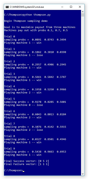
A good way to see where this article is headed is to look at the screenshot of a demo run in Figure 1. The demo sets up three machine that pay out with probabilities (0.3, 0.7, 0.5) respectively. Therefore, machine [0] is the worst and machine [1] is the best. These probabilities would be unknown to you in a real problem. On each of the 10 trials, three probability values are generated, and the machine with the highest probability is played. Generating these probabilities uses the mathematical beta distribution and is the key to Thompson Sampling.
On each trial, the selected machine is played and either wins (a success) or loses (a failure). The current number of successes and failures for each machine are used to determine the probability values. At the end of the demo run, machine [0] won 0 times and lost 1 time; machine [1] won 5 times and lost 1 time; machine [2] won 2 times and lost 1 time. In this simulation, the best machine was correctly identified, and with 7 wins and 3 losses, there was a net gain of 4.
 [Click on image for larger view.]
Figure 1. Thompson Sampling Demo Run
This article assumes you have intermediate or better programming skill with Python or a C-family language but doesn't assume you know anything about Thompson Sampling. The complete demo code is presented in this article.
Understanding the Beta Distribution
There are many probability distributions. You've likely encountered Gaussian (also called normal, or bell-shaped) distributions. A Gaussian distribution is characterized by two values, the mean and the standard deviation. Different values of mean and standard deviation generate different behaviors. For example, if you sampled 1,000 times from a Gaussian distribution with mean = 0.0 and standard deviation = 1.0, you'd expect about 380 results between -0.5 and +0.5.
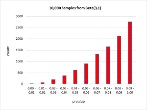
The beta distribution is also characterized by two values. They don't have names and are usually called alpha and beta, or just a and b. Notice there's a possible source of confusion between "beta" as the name of the distribution and "beta" as one of the two characteristic values. A beta distribution with a = 1 and b = 1 behaves like flipping a coin. You'll get values between 0.0 and 1.0 but the values will average to 0.5. In general, the average value from a beta distribution with characteristic values a and b will be a / (a + b). For example, the average value returned from beta with a = 3 and b = 1 is 3 / (3 + 1) = 0.75. A graph of 10,000 samples from beta(3, 1) is shown in Figure 2.
 [Click on image for larger view.]
Figure 1. Sampling from the Beta(3, 1) Distribution
It's not entirely obvious how the beta distribution is related to a multi-armed bandit problem. Suppose at some point in a multi-armed bandit problem with just two machines, machine [0] has 3 successes and 2 failures, and machine [1] has 5 successes and 1 failure. You'd guess that the probability that machine [0] pays out is 3 / 5 = 0.60 and the probability that machine [1] pays out is 5 / 6 = 0.83. So you be inclined to play machine [1]. But you still want to have a chance of playing machine [0] just in case it's actually the best machine and you've been unlucky so far.
Sampling from the beta distribution will generate probabilities where the machine with the best success to failure ratio will usually have the largest probability, but there'll still be a chance for a machine with a lower ratio to generate the largest probability. Very, very clever.
The Demo Program
The complete demo program, with a few minor edits to save space, is presented in Listing 1. I used the most excellent Notepad to edit my program but most of my colleagues prefer something a bit more powerful such as Visual Studio Code. I indent with two spaces instead of the usual four to save space.
Listing 1: The Thompson Sampling Demo Program
# thompson.py
# Python 3.6.5

import numpy as np

def main():
  print("Begin Thompson sampling demo ")
  print("Goal is to maximize payout from three machines")
  print("Machines pay out with probs 0.3, 0.7, 0.5")

  N = 3  # number machines
  means = np.array([0.3, 0.7, 0.5])
  probs = np.zeros(N)
  S = np.zeros(N, dtype=np.int)
  F = np.zeros(N, dtype=np.int)
  rnd = np.random.RandomState(7)

  for trial in range(10):
    print("\nTrial " + str(trial))

    for i in range(N):
      probs[i] = rnd.beta(S[i] + 1, F[i] + 1)

    print("sampling probs =  ", end="")
    for i in range(N):
      print("%0.4f  " % probs[i], end="")
    print("")

    machine = np.argmax(probs)
    print("Playing machine " + str(machine), end="")

    p = rnd.random_sample()  # [0.0, 1.0)
    if p < means[machine]:
      print(" -- win")
      S[machine] += 1
    else:
      print(" -- lose")
      F[machine] += 1

  print("Final Success vector: ", end="")
  print(S)
  print("Final Failure vector: ", end="")
  print(F)

if __name__ == "__main__":
  main()
All normal error-checking has been omitted to keep the main ideas as clear as possible. I used Python version 3.6.5 with NumPy version 1.14.3 but any relatively recent versions will work fine.
The demo begins with these six statements:
N = 3
means = np.array([0.3, 0.7, 0.5])
probs = np.zeros(N)
S = np.zeros(N, dtype=np.int)
F = np.zeros(N, dtype=np.int)
rnd = np.random.RandomState(7)
Variable N is the number of machines. The array named means holds the probabilities that each machine will pay out. Because machines pay out either 0 or 1, this is an example of a Bernoulli multi-armed bandit. There are other types of problems but Bernoulli is the most common. The array named probs holds the probabilities generated at each trial. Arrays S and F hold the cumulative number of successes and failures of each machine at any point in time. Object rnd is used to sample from the beta distribution and is also used to determine if a selected machine wins or loses. The seed value, 7, was used only because it gave a representative demo run.
The demo program consists mostly of a single for-loop. Inside the loop, the first step is to generate sampling probabilities from the beta distribution for each machine, using each machine's count of successes and failures:
for trial in range(10):
  print("Trial " + str(trial))

  for i in range(N):  # each machine
    probs[i] = rnd.beta(S[i] + 1, F[i] + 1)
. . .
The built-in NumPy beta(a, b) function draws a sample from the beta distribution. Here the function call adds 1 to each a (success) and b (failure) count because beta(a, b) requires that a and b be strictly greater than 0. Having a built-in Python beta() function is very convenient. If you're implementing Thompson Sampling in most other programming languages, you'll have to find an external library, or implement a beta() function yourself. The code in Listing 2 presents a raw Python implementation of a beta sampling class to give you an idea of what is involved.
Listing 2: A Program-Defined Beta Sampling Class
class BetaSampler:
  def __init__(self, seed):
    self.rnd = np.random.RandomState(seed)

  def next_sample(self, a, b):
    # a, b > 0
    alpha = a + b
    beta = 0.0
    u1 = 0.0; u2 = 0.0; w = 0.0; v = 0.0

    if min(a, b) <= 1.0:
      beta = max(1 / a, 1 / b)
    else:
      beta = np.sqrt((alpha - 2.0) / (2 * a * b - alpha))
    gamma = a + 1 / beta

    while True:
      u1 = self.rnd.random_sample()
      u2 = self.rnd.random_sample()
      v = beta * np.log(u1 / (1 - u1))
      w = a * np.exp(v)
      tmp = np.log(alpha / (b + w))
      if alpha * tmp + (gamma * v) - 1.3862944 >= \
        np.log(u1 * u1 * u2):
        break
    x = w / (b + w)
    return x
After generating beta probabilities, the demo determines which probability is the largest using the handy argmax() function. The selected machine is virtually played by calling the random_sample() function which returns a value between 0.0 and 1.0. For example, the probability that machine [0] wins is 0.3. If the return result from random_sample() is less than 0.3 then the machine wins, otherwise the machine loses.
Wrapping Up
Multi-armed bandit problems are often considered part of what's called reinforcement learning. But some of my colleagues categorize multi-armed bandit problems as distinct one-of-a-kind type of problems. Briefly, supervised learning requires training data that has known correct answers. Most forms of neural networks use supervised learning techniques. Unsupervised learning uses data but does not require known correct answers. Data clustering is an example of unsupervised learning. Reinforcement learning does not use explicit data, instead, a prediction model is created using feedback from a reward function of some sort.
About the Author
Dr. James McCaffrey works for Microsoft Research in Redmond, Wash. He has worked on several Microsoft products including Azure and Bing. James can be reached at [email protected].