The Data Science Lab
Working With PyTorch Tensors
Dr. James McCaffrey of Microsoft Research presents the fundamental concepts of tensors necessary to establish a solid foundation for learning how to create PyTorch neural networks, based on his teaching many PyTorch training classes at work.
PyTorch is a Python language code library that can be used to create deep neural networks. The fundamental object in PyTorch is called a tensor. A tensor is essentially an n-dimensional array that can be processed using either a CPU or a GPU.
PyTorch tensors are surprisingly complex. One of the keys to getting started with PyTorch is learning just enough about tensors, without getting bogged down with too many details. With a basic knowledge of tensors in hand you can learn how to create and use neural networks in a spiral manner, adding knowledge of details with each new program you write.
This article presents what I consider (based on teaching many PyTorch training classes at my workplace) the fundamental concepts of tensors necessary to establish a solid foundation for learning how to create PyTorch neural networks.
The screenshot in Figure 1 and the code in Listing 1 show a minimal "hello world" PyTorch neural network. The idea is to provide you with some context for how tensors are used in practice.
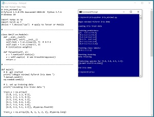 [Click on image for larger view.] Figure 1: A Minimal PyTorch Neural Network in Action
The demo program creates a neural network that predicts the species of an iris flower (setosa = 0, versicolor = 1, or virginica = 2) based on four predictor values (sepal length and width, petal length and width). All of the input values, internal processing values, and output values are stored in PyTorch tensors.
Listing1: A Minimal PyTorch Neural Network
# iris_minimal.py
# PyTorch 1.5.0-CPU Anaconda3-2020.02 Python 3.7.6
# Windows 10

import numpy as np
import torch as T
device = T.device("cpu")

# -------------------------------------------------

class Net(T.nn.Module):
  def __init__(self):
    super(Net, self).__init__()
    self.hid1 = T.nn.Linear(4, 7)  # 4-7-3
    self.oupt = T.nn.Linear(7, 3)
    # (initialize weights)

  def forward(self, x):
    z = T.tanh(self.hid1(x))
    z = self.oupt(z)  # see CrossEntropyLoss()
    return z

# -------------------------------------------------

def main():
  # 0. get started
  print("\nBegin minimal PyTorch Iris demo ")
  T.manual_seed(1)
  np.random.seed(1)

  # 1. set up training data in tensors
  print("\nLoading Iris train data ")

  train_x = np.array([
    [5.0, 3.5, 1.3, 0.3],
    [4.5, 2.3, 1.3, 0.3],
    [5.5, 2.6, 4.4, 1.2],
    [6.1, 3.0, 4.6, 1.4],
    [6.7, 3.1, 5.6, 2.4],
    [6.9, 3.1, 5.1, 2.3]], dtype=np.float32)

  train_y = np.array([0, 0, 1, 1, 2, 2],
    dtype=np.long)

  print("\nTraining predictors:")
  print(train_x)
  print("\nTraining class labels: ")
  print(train_y)

  train_x = T.tensor(train_x,
    dtype=T.float32).to(device)
  train_y = T.tensor(train_y,
    dtype=T.long).to(device)

  # 2. create network
  net = Net().to(device)

  # 3. train model
  max_epochs = 100
  lrn_rate = 0.04
  loss_func = T.nn.CrossEntropyLoss()
  optimizer = T.optim.SGD(net.parameters(),
    lr=lrn_rate)

  print("\nStarting training ")
  net.train()
  indices = np.arange(6)
  for epoch in range(0, max_epochs):
    np.random.shuffle(indices)
    for i in indices:
      X = train_x[i].reshape(1,4)
      Y = train_y[i].flatten()
      optimizer.zero_grad()
      oupt = net(X)
      loss_obj = loss_func(oupt, Y)
      loss_obj.backward()
      optimizer.step()
    # (monitor error)
  print("Done training ")

  # 4. use model to make a prediction
  net.eval()
  print("\nPredicting for [5.8, 2.8, 4.5, 1.3]: ")
  unk = np.array([[5.8, 2.8, 4.5, 1.3]],
    dtype=np.float32)
  unk = T.tensor(unk, dtype=T.float32).to(device)
  logits = net(unk).to(device)
  probs = T.nn.functional.softmax(logits, dim=1)
  probs = probs.detach().numpy()  # nicer printing

  np.set_printoptions(precision=4)
  print(probs)

  print("\nEnd Iris demo")

if __name__ == "__main__":
  main()
If you scan through the code listing you'll see several statements where tensors are explicitly created using the tensor() constructor. Tensors are also implicitly created by calls to Linear() in the neural network class constructor, and as return values from reshape(), flatten(), tanh(), softmax(), and other functions.
In order to get the demo program to run on your machine, you must install PyTorch. This is not trivial. The installation process is covered in detail in the previous Visual Studio Magazine Data Science Lab article "Getting Started with PyTorch 1.5 on Windows."
This article assumes you have intermediate or better programming skill with a C-family language (preferably but not necessarily Python) but doesn't assume you know anything about PyTorch tensors.
Creating Tensors
The demo program in Listing 2 presents examples of fundamental operations on PyTorch tensors. Basic operations include creating tensors, reshaping tensors, and calling functions that accept tensors as arguments. Although the demo program is short, it is extremely dense in terms of tensor concepts.
Listing 2: Basic PyTorch Tensor Operations
# tensor_examples.py
# PyTorch 1.5.0-CPU Anaconda3-2020.02 Python 3.7.6
# Windows 10

import numpy as np
import torch as T
device = T.device("cpu")

# -------------------------------------------------

def main():
  print("\nBegin PyTorch tensor examples ")

  np.random.seed(1)
  T.manual_seed(1)
  T.set_printoptions(precision=2)

  # 1. creating from numpy or list

  a1 = np.array([[0, 1, 2],
                 [3, 4, 7]], dtype=np.float32)
  t1 = T.tensor(a1, dtype=T.float32).to(device)
  t2 = T.tensor([0, 1, 2, 3],
    dtype=T.int64).to(device)
  t3 = T.zeros((3,4), dtype=T.float32)
  x = t1[1][0]  # [3.0] tensor float32
  v = x.item()  # 3.0 scalar

  # 2. shape, reshape, view, flatten, squeeze

  print(t1.shape)         # torch.Size([2, 3])
  t4 = t1.reshape(1,3,2)  # or t1.view(1,3,2)
  t5 = t1.flatten()       # or T.flatten(t1)
  t6 = t4.squeeze()       # or T.reshape(t4, (3,-1))

  # 3. tensor to numpy or list

  a2 = t1.numpy()         # t1.detach().numpy()
  lst1 = t1.tolist()

  # 4. functions

  t7 = T.add(t1, 2.5)    # t7 = t1 + 2.5
  t7.add_(3.5)

  (big_vals, big_idxs) = T.max(t1, dim=1)
  print(big_vals)  # [2, 7]

  probs = T.softmax(t1, dim=1)
  print(probs[0])

  print("\nEnd demo ")

# -------------------------------------------------

if __name__ == "__main__":
  main()
The demo program begins with these statements:
# tensor_examples.py
# PyTorch 1.5.0-CPU Anaconda3-2020.02 Python 3.7.6
# Windows 10

import numpy as np
import torch as T
device = T.device("cpu")
. . .
The PyTorch library has been under continuous revision since its creation so it's important to document which version is being used, as well as the associated Python version and operating system platform. Every non-trivial PyTorch program uses the NumPy library so it's almost always imported with alias np.
PyTorch is imported as "torch" rather than "pytorch" as you might expect because PyTorch is based on the C++ language Torch library. For reasons which aren't at all clear to me, unlike almost every other Python module, PyTorch is rarely assigned an alias. Therefore, the alias of T used in the demo is not one you'll see often, even though it makes PyTorch programs easier to read in my opinion.
I recommend including a program-global device definition in all PyTorch programs. This allows you to easily toggle between targeting a CPU machine and a GPU machine, by changing the device to T.device("cuda").
The demo places all control statements in a main() function:
def main():
  print("\nBegin PyTorch tensor examples ")

  np.random.seed(1)
  T.manual_seed(1)
  T.set_printoptions(precision=2)
. . .
I recommend beginning all PyTorch programs by setting seed values for the NumPy and PyTorch random number generators. Although they're not needed by the tensor examples demo program, almost all non-trivial PyTorch programs use randomness when training a neural network. The call to set_printoptions() tells the demo to display tensor values to two decimals.
The demo shows four ways to create a PyTorch tensor:
  a1 = np.array([[0, 1, 2],
                 [3, 4, 7]], dtype=np.float32)
  t1 = T.tensor(a1, dtype=T.float32).to(device)
  t2 = T.tensor([0, 1, 2, 3],
    dtype=T.int64).to(device)
  t3 = T.zeros((3,4), dtype=T.float32)
  x = t1[1][0]  # [3.0] tensor float32
  v = x.item()  # 3.0 scalar
. . .
Tensor t1 is created by first generating a NumPy array named a1 and then passing the array to the tensor() constructor. The two most common data types used by PyTorch are float32 and int64. PyTorch supports nine atomic data types as shown in the table in Figure 2.
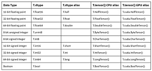 [Click on image for larger view.]Figure 2: The Nine PyTorch Data Types
The statement that creates tensor t1 has a ".to(device)" call appended. In most cases you should specify the device on all statements that explicitly create a tensor. Tensors that are created implicitly, such as return objects from functions, inherit the device of the argument tensor(s) so you don't need to specify the device on such statements.
Tensor t2 is created by passing a Python list of [1, 2, 3, 4] to the tensor() constructor. Compared to other code libraries and programming languages, PyTorch has a huge number of aliases. For example, tensor t2 could have been created by the statement t2 = T.LongTensor([1,2,3,4]).to(device). Dealing with the crazy number of aliases and default parameter values in PyTorch is a significant challenge.
Tensor t3 is created by the statement t3 = T.zeros((3,4), dtype=T.float32).to(device). Tensor t3 is a 3x4 2-dimensional tensor. You can loosely think of t3 as having 3 rows and 4 columns even though, technically, that's not entirely correct.
A value is fetched from tensor t1 by the statement x = t1[1][0] which loosely means the value at row [1] and column [0]. The result x is not a float32 scalar value as you might expect. Instead, x is a one-dimensional tensor holding a single 3.0 value. To fetch the scalar value from a tensor you can use the item() function, such as v = x.item() in the demo.
One of the optional parameters of the tensor() constructor is requires_grad. The default value is False. Only tensors that hold neural network weights and biases, and are therefore updated using some form of gradient descent, need the requires_grad parameter set to True. In most cases, such as when you use the T.nn.Module class and tensors are created implicitly, the requires_grad parameter is handled for you.
Prior to version 0.4 PyTorch contained a Variable object that was much like a Tensor object. A Variable had a gradient but a Tensor didn't. The gradient functionality of the old Variable type was added to the Tensor type, so if you see example code with a Variable object, the example is out of date and you should consider looking for a newer example.
Reshaping Tensors
Somewhat surprisingly, almost all non-demo PyTorch programs require you to reshape tensors. Dealing with tensor shapes is trickier than you might expect. The four basic reshaping functions are reshape(), view(), flatten(), and squeeze(). The demo program illustrates reshaping functions with these statements:
  print(t1.shape)         # or t1.size() = torch.Size([2, 3])
  t4 = t1.reshape(1,3,2)  # or t1.view(1,3,2)
  t5 = t1.flatten()       # or T.flatten(t1)
  t6 = t4.squeeze()       # or T.reshape(t4, (3,-1))
. . .
The shape property (notice no parentheses) returns the shape of its associated tensor. You can also use the exactly equivalent size() method. Both give the shape of the tensor t1 as Size[2, 3] which can be interpreted as 2x3. Therefore, tensor t1 is 2-dimensional and has six elements.
The statement t4 = t1.reshape(1,3,2) produces a tensor t4 which has the same six elements as t1, but in a 3-dimensional tensor. Another example would be t4 = t1.reshape(3,2). But t4 = t1.reshape(4,2) would be an error because the statement is asking for eight elements instead of six.
The view() function is almost exactly the same as the reshape() function. For example, the statements t = t.reshape(2,7,4) and t = t.view(2,7,4) both create a 2x7x4 3-dimensional tensor. The difference is that the view() function requires that the associated tensor have values that are stored contiguously in memory, but reshape() allows tensor values to be stored either contiguously or in different areas of memory. In most cases I use reshape() rather than view() so I don't have to check the tensor using a call to the is_contiguous() function.
The flatten() function reshapes a tensor with two or more dimensions into a 1-dimensional tensor. The statement t5 = t1.flatten() in the demo program takes 2-dimensional tensor t1, which has shape [2,3] and creates a 1-dimensional tensor t5 that has shape [6], which means 6 elements. The same tensor could have been created by the statement t5 = t1.reshape(6).
The squeeze() function is best explained by example. Suppose you create a 5-dimensional tensor with the statement t1 = T.zeros((4,1,3,1,7), dtype=T.float32).to(device). The statement t2 = t1.squeeze() creates a tensor with shape [4,3,7]. If you think about it carefully, you'll realize that any dimension that has size 1 is useless in some sense because you can only index it with [0]. For example, if t1 = T.zeros((3,4,1), dtype=T.float32).to(device) then you can access a value with a statement like x = t1[2][3][0]. The last index must always be [0]. The squeeze() function removes such dimensions.
When reshaping tensors, you can specify a -1 for one of the shape values, which means "figure the value out for me". For example, suppose a tensor t1 has shape [3,4,5]. The tensor has 60 elements. The statement t2 = t1.reshape(10, -1) creates t2 with shape [10, 6]. Using -1 for a reshape value is usually done inside a loop where the shape of the source tensor changes, for example when the source tensor is a batch of training items and the last batch can be smaller than all the other batches.
Converting Tensors and Tensors are Reference Objects
The demo program shows examples of converting a PyTorch tensor to a NumPy array and a Python list:
  a2 = t1.numpy()
  lst1 = t1.tolist()
. . .
The most common use of the numpy() and tolist() functions occurs at the end of a PyTorch neural network program, so that the resulting array or list can be used by some other system. In most cases it's not a good idea to convert tensors to an array or list, process the array or list, then convert back to a tensor. This approach is inefficient and in almost all scenarios you can just operate on tensors directly.
Many, but not all, tensors are part of a neural network. Technically a PyTorch neural network is called a computational graph. For such tensors, if you attempt to convert to a NumPy array you will get an error. To avoid this error you must use the detach() function, for example, arr = t1.detach().numpy(). See the program in Listing 1 for a realistic example.
Tensors are reference objects. An important implication is that you must be careful when using tensors in assignment statements and as function parameters. For example, consider this code:
t1 = T.tensor([1.0, 2.0, 3.0],
  dtype=T.float32).to(device)
t2 = t1
t3 = t1.clone()
t1[1] = 9.0
Tensor t2 is a reference to tensor t1 so changing cell [1] of t1 to 9.0 also changes cell [1] of tensor t2. Tensor t3 is a true copy of t1 so the change made to t1 has no effect on t3.
When a tensor is used as a function parameter, the function can change the tensor. For example:
def foo(some_tensor):
  some_tensor *= 2
  return -1

t1 = T.tensor([1.0, 2.0, 3.0], dtype=T.float32).to(device)
result = foo(t1)
The call to foo() will multiply all values in tensor t1 by 2 so t1 will hold [2.0, 4.0, 6.0] after the call.
Tensor Functions
The demo program concludes by showing four examples of tensor functions:
. . .
  t7 = T.add(t1, 2.5)    # t7 = t1 + 2.5
  t7.add_(3.5)

  (big_vals, big_idxs) = T.max(t1, dim=1)
  print(big_vals)  # [2, 7]

  probs = T.softmax(t1, dim=1)
  print(probs[0])
  print("\nEnd demo ")
if __name__ == "__main__":
  main()
Recall that t1 is a 2x3 tensor with float32 values:
[[0, 1, 2],
 [3, 4, 7]]
The statement t7 = T.add(t1, 2.5) adds 2.5 to each element of t1 giving:
[[2.5, 3.5, 4.5],
 [5.5, 6.5, 9.5]]
The statement t7.add_(3.5) adds 3.5 to each element of t7 giving:
[[6.0,  7.0,  8.0],
 [9.0, 10.0, 13.0]]
By convention, PyTorch functions that have names with a trailing underscore operate in-place rather than returning a value. The use of an in-place function is relatively rare and is most often used with very large tensors to save memory space.
The statement (big_vals, big_idxs) = T.max(t1, dim=1) returns two values. Variable big_vals holds the largest values in the two rows of t1, which are [2, 7] -- 2 is the largest value in the first row and 7 is the largest value in the second row. The big_idxs variable holds the indices of the largest values in each row and so is [2, 2].
If the dim parameter was set dim=0 the result would be [3, 4, 7] -- the largest values in each column. Many PyTorch tensor functions accept a dim parameter. Working with dim parameters is a bit trickier than the demo examples suggest. A dim value doesn't really specify "row" or "column" but for 2-dimensional tensors you can usually think about the dim parameter in this way.
The mathematical softmax() function accepts a vector of values and scales them so that they sum to 1.0 and can then be loosely interpreted as probabilities. The demo program statement probs = T.softmax(t1, dim=1) returns the softmax values for both the first row and second row of tensor t1 stored as:
[[0.09, 0.24, 0.67],
 [0.02, 0.05, 0.94]]
Therefore probs[0] holds the softmax values for the first row = [0.09, 0.24, 0.67].
If the dim parameter was set dim=0 the result would be the softmax values for the first, second, and third columns of t1. The softmax values of the first column of t1 are [0.05, 0.95], the softmax values of the second column of t1 are also [0.05, 0.95], and the softmax values of the third column of t1 are [0.01, 0.99]. However, the return values are stored as:
[[0.05, 0.05, 0.01],
 [0.95, 0.95, 0.99]]
Therefore, probs[0] is [0.05, 0.05, 0.01] which has no meaning. The moral of the story is that you should be very careful when working with tensor functions that have a dim parameter.
Flexibility and Controlled Chaos
An optimist might say that PyTorch gives you tremendous flexibility by having multiple ways to do most tasks. A pessimist might say that the evolution of PyTorch was not controlled very well, resulting in a ridiculous number of ways to do most tasks. Regardless, dealing with the large number of ways to do most tasks is a significant challenge because no two examples will be the same.
For example, the following seven statements all create the identical float32 tensor t:
t = T.tensor([1, 2, 3], dtype=T.float).to(device)
t = T.tensor([1, 2, 3], dtype=T.float32).to(device)
t = T.tensor([1, 2, 3], dtype=T.float32,
  requires_grad=False).to(device)
t = T.tensor([1.0, 2.0, 3.0]).to(device)
t = T.FloatTensor([1, 2, 3]).to(device)
t = T.Tensor([1, 2, 3]).to(device)
t = T.from_numpy( np.array([1, 2, 3],
  dtype=np.float32) ).to(device)
However, the following statement which is almost the same creates a completely different int64 tensor:
t = T.tensor([1, 2, 3]).to(device)
Many PyTorch functions can be called as either static or instance. For example, the following two statements create the same tensor:
t2 = t1.reshape(3,4)       # instance
t2 = T.reshape(t1, (3,4))  # static
Over time, different versions of the same function have emerged in different modules. For example, the following statements use three different PyTorch softmax functions to generate the identical result:
t1 = T.tensor([1, 2, 3], dtype=T.float32).to(device)
p = T.softmax(t1, dim=0)
p = T.nn.functional.softmax(t1, dim=0)
p = T.nn.Softmax(dim=0)(t1)
PyTorch is very permissive with syntax. For example, the following four statements all create a 1-dimensional tensor initialized to three random float32 values between 0.0 and 1.0:
t1 = T.rand((3), dtype=T.float32).to(device)
t1 = T.rand(3, dtype=T.float32).to(device)
t1 = T.rand((3,), dtype=T.float32).to(device)
t1 = T.rand([3], dtype=T.float32).to(device)
The bottom line is that dealing with multiple ways to perform a task in PyTorch is a challenge you shouldn't underestimate. This means that being consistent with your coding patterns, such as always using T.float32 rather than the T.float alias, and commenting your PyTorch code, is very important.
Wrapping Up
I regularly use PyTorch, as well as the TensorFlow and Keras neural code libraries, and the scikit-learn library. And for single hidden layer neural networks I often implement from scratch using C, C#, Java, or Python. All these approaches have strengths and weaknesses. That said, I particularly like using PyTorch. PyTorch has a significant learning curve, but after getting over initial hurdles such as working with tensors, PyTorch provides you with an excellent combination of power and flexibility.