The Data Science Lab
Regression Using scikit Kernel Ridge Regression
A regression problem is one where the goal is to predict a single numeric value. For example, you might want to predict the annual income of a person based on their sex, age, State where they live and political leaning. Note that the common "logistic regression" machine learning technique is a binary classification system in spite of its name.
There are many different techniques available to create a regression model. Some common techniques, listed from less complex to more complex, are: linear regression, linear lasso regression, linear ridge regression, k-nearest neighbors regression, (plain) kernel regression, kernel ridge regression, Gaussian process regression, decision tree regression and neural network regression. This article explains how to create and use kernel ridge regression (KRR) models. Compared to other regression techniques, KRR is especially useful when there is limited training data.
There are several tools and code libraries that you can use to create a KRR regression model. The scikit-learn library (also called scikit or sklearn) is based on the Python language and is one of the most popular.
A good way to see where this article is headed is to take a look at the screenshot in Figure 1. The demo program loads a 200-item set of training data and a 40-item set of test data into memory. Next, the demo creates and trains a KRR model using the scikit KernelRidge module.
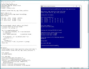 [Click on image for larger view.] Figure 1: Kernel Ridge Regression in Action
After training, the model is applied to the training data and the test data. The model scores 88 percent accuracy (176 out of 200) on the training data, and 80 percent accuracy (32 out of 40) on the test data. The demo program defines a correct income prediction as one that's within 10 percent of the true income.
The demo concludes by predicting the income of a new, previously unseen person who is male, age 34, from Oklahoma, and who is a political moderate. The predicted income is $45,460.44.
This article assumes you have intermediate or better skill with a C-family programming language, but doesn't assume you know much about kernel ridge regression or the scikit library. The complete source code for the demo program is presented in this article and in the accompanying file download. The source code and data are also available online.
Installing the scikit Library
There are several ways to install the scikit library. I recommend installing the Anaconda Python distribution. Anaconda contains a core Python engine plus over 500 libraries that are (mostly) compatible with each other. I used Anaconda3-2022.10 which contains Python 3.9.13 and the scikit 1.0.2 version. The demo code runs on Windows 10 or 11.
Briefly, Anaconda / Python / scikit is installed using a Windows self-extracting executable file. The setup process is mostly straightforward and takes about 15 minutes following step-by-step instructions.
There are more up-to-date versions of Anaconda / Python / scikit library available. But because the Python ecosystem has hundreds of libraries, if you install the most recent versions of these libraries, you run a greater risk of library incompatibilities -- a major headache when working with Python.
The Data
The data is artificial. There are 200 training items and 40 test items. The structure of data looks like:
 1   0.24   1 0 0   0.2950   0 0 1
 0   0.39   0 0 1   0.5120   0 1 0
 1   0.63   0 1 0   0.7580   1 0 0
 0   0.36   1 0 0   0.4450   0 1 0
 1   0.27   0 1 0   0.2860   0 0 1
. . .
The tab-delimited fields are sex (0 = male, 1 = female), age (divided by 100), State (Michigan = 100, Nebraska = 010, Oklahoma = 001), income (divided by $100,000) and political leaning (conservative = 100, moderate = 010, liberal = 001).
Kernel ridge regression was originally designed for problems with strictly numeric predictor variables. However, KRR can be applied to problems with categorical data as demonstrated in this article.
Based on my experience with KRR, the numeric predictors should be normalized to all the same range -- typically 0.0 to 1.0 or -1.0 to +1.0 -- because normalizing can prevent predictors with large magnitudes from overwhelming those with small magnitudes.
For categorical predictor variables, I recommend one-hot encoding. For example, if there were five states instead of just three, the states would be encoded as 10000, 01000, 00100, 00010, 00001.
Understanding Kernel Ridge Regression
A good way to understand kernel ridge regression is to examine a concrete example. Suppose your training data has just four items where each predictor value is a vector with size = 3, and the target value to predict is a single floating-point value. For example:
x0 = (0.1, 0.5, 0.2)  y0 = 0.3
x1 = (0.4, 0.3, 0.0)  y1 = 0.9
x2 = (0.6, 0.1, 0.8)  y2 = 0.4
x3 = (0.0, 0.2, 0.7)  y3 = 0.8
A kernel function accepts two vectors and returns a value that is a measure of similarity/dissimilarity. There are many possible kernel functions and each type has several variations. One of the most common kernel functions is the radial basis function. A common version is defined as rbf(a, b, gamma) = exp(-gamma * ||a - b||^2). The ||a - b||^2 term is the squared Euclidean distance between vectors a and b. For example:
rbf(x0, x1, 1.0)
 = exp( -1 * (0.1-0.4)^2 + (0.5-0.3)^2 + (0.2-0.0)^2 )
 = exp( -1 * (0.09 + 0.04 + 0.04) )
 = exp(-0.17)
 = 0.8437
A trained KRR model produces one weight per training item. The weights are sometimes called the dual coefficients. Suppose the weights are (w0, w1, w2, w3) = (-3.7, 3.3, -1.2, 2.5). The predicted y for a new x is the sum of the weights times the kernel function applied to x and each training vector. Suppose x = (0.5, 0.4, 0.6), then (subject to rounding):
y_pred = w0 * rbf(x, x0, 1.0) +
         w1 * rbf(x, x1, 1.0) +
         w2 * rbf(x, x2, 1.0) +
         w3 * rbf(x, x3, 1.0)

       = -3.7 * rbf(x, x0, 1.0) +
          3.3 * rbf(x, x1, 1.0) +
         -1.2 * rbf(x, x2, 1.0) +
          2.5 * rbf(x, x3, 1.0)

       = -3.7 * 0.72 +
          3.3 * 0.69 +
         -1.2 * 0.87 +
          2.5 * 0.74

        = -2.6 + 2.2 + -1.0 + 1.8

        =  0.40
The scikit KernelRidge model weights are computed behind the scenes using matrix algebra.
The Demo Program
The complete demo program is presented in Listing 1. Notepad is my preferred code editor but most of my colleagues prefer one of the many excellent IDEs that are available for Python. I indent my Python program using two spaces rather than the more common four spaces.
The program imports the NumPy library, which contains numeric array functionality, the KernelRidge module, which contains kernel ridge regression functionality, and the pickle module, which is used for saving a trained model. Notice the name of the root scikit module is sklearn rather than scikit.
import numpy as np
from sklearn.kernel_ridge import KernelRidge
import pickle
In terms of Python style, I prefer to place all the import statements at the top of a program. An alternative is to place each import statement near its first usage.
Listing 1: Complete Demo Program
# kernel_ridge_regression.py
# Anaconda3-2022.10  Python 3.9.13
# Windows 10/11
# scikit / sklearn 1.0.2

# predict income from sex, age, State, politics

import numpy as np
from sklearn.kernel_ridge import KernelRidge
import pickle

# sex age   state   income   politics
#  0  0.27  0 1 0   0.7610   0 0 1
#  1  0.19  0 0 1   0.6550   1 0 0

# -----------------------------------------------------------

def accuracy(model, data_X, data_y, pct_close):
  # correct within pct of true income
  n_correct = 0; n_wrong = 0

  for i in range(len(data_X)):
    X = data_X[i].reshape(1, -1)  # one-item batch
    y = data_y[i]
    pred = model.predict(X)       # predicted income

    if np.abs(pred - y) < np.abs(pct_close * y):
      n_correct += 1
    else:
      n_wrong += 1
  acc = (n_correct * 1.0) / (n_correct + n_wrong)
  return acc

# -----------------------------------------------------------

def main():
  print("\nBegin kernel ridge regression using scikit demo ")
  print("Predict income from sex, age, State, political ")

  # 0. prepare
  np.random.seed(1)

  # 1. load data
  print("\nLoading data into memory ")
  train_file = ".\\Data\\people_train.txt"
  train_xy = np.loadtxt(train_file, delimiter="\t",
    usecols=[0,1,2,3,4,5,6,7,8], comments="#",
    dtype=np.float64)
  train_X = train_xy[:,[0,1,2,3,4,6,7,8]]
  train_y = train_xy[:,5].flatten()  # 1D required

  print("\nFirst four X predictors = ")
  print(train_X[0:4,:])
  print(" . . . ")
  print("\nFirst four target y = ")
  print(train_y[0:4])
  print(" . . . ")

  test_file = ".\\Data\\people_test.txt"
  test_xy = np.loadtxt(test_file, delimiter="\t",
    usecols=[0,1,2,3,4,5,6,7,8], comments="#",
    dtype=np.float64)
  test_X = test_xy[:,[0,1,2,3,4,6,7,8]]
  test_y = test_xy[:,5].flatten()  # 1D required

# -----------------------------------------------------------

  # 2. create and train KRR model
  print("\nCreating and training KRR RBF(1.0) model ")
  # KernelRidge(alpha=1.0, *, kernel='linear', gamma=None,
  #   degree=3, coef0=1, kernel_params=None)
  # ['additive_chi2', 'chi2', 'linear', 'poly', 'polynomial',
  #  'rbf', 'laplacian', 'sigmoid', 'cosine']

  # model = KernelRidge(alpha=1.0, kernel='poly', degree=4)
  model = KernelRidge(alpha=0.1, kernel='rbf', gamma=1.0)
  model.fit(train_X, train_y)

  # 3. compute model accuracy
  print("\nComputing accuracy (within 0.10 of true) ")
  acc_train = accuracy(model, train_X, train_y, 0.10)
  print("Accuracy on train data = %0.4f " % acc_train)
  acc_test = accuracy(model, test_X, test_y, 0.10)
  print("Accuracy on test data = %0.4f " % acc_test)

  # 4. make a prediction
  print("\nPredicting income for M 34 Oklahoma moderate: ")
  X = np.array([[0, 0.34, 0,0,1,  0,1,0]],
    dtype=np.float32)
  pred_inc = model.predict(X)
  print("$%0.2f" % (pred_inc * 100_000))  # un-normalized

  # 5. save model
  print("\nSaving model ")
  fn = ".\\Models\\krr_model.pkl"
  with open(fn,'wb') as f:
    pickle.dump(model, f)

  # load model
  # with open(fn, 'rb') as f:
  #   loaded_model = pickle.load(f)
  # pi = loaded_model.predict(X)
  # print("%0.2f" % (pi * 100_000))  # un-normalized

  print("\nEnd scikit KRR demo ")

if __name__ == "__main__":
  main()
All the program logic is contained in a main() function. The demo defines an accuracy() function that emphasizes clarity at the expense of efficiency. The demo begins by setting the NumPy random seed:
def main():
  print("Begin kernel ridge regression using scikit demo ")
  print("Predict income from sex, age, State, political ")
  # 0. prepare
  np.random.seed(1)
 . . .
Technically, setting the random seed value isn't necessary, but doing so helps you to get reproducible results in many situations where there are one or more random components. The KernelRidge module doesn't have any random components, but setting the seed is good practice in my opinion.
Loading the Training and Test Data
The demo program loads the training data into memory using these statements:
  # 1. load data
  print("Loading data into memory ")
  train_file = ".\\Data\\people_train.txt"
  train_xy = np.loadtxt(train_file, delimiter="\t",
    usecols=[0,1,2,3,4,5,6,7,8], comments="#",
    dtype=np.float64)
  train_X = train_xy[:,[0,1,2,3,4,6,7,8]]
  train_y = train_xy[:,5].flatten()  # 1D required
This code assumes the data files are stored in a directory named Data. There are many ways to load data into memory. I prefer using the NumPy library loadtxt() function, but a common alternative is the Pandas library read_csv() function.
The code reads all 200 lines of training data (columns 0 to 8 inclusive) into a matrix named train_xy and then splits the data into a matrix of predictor values and a vector of target income values. The colon syntax means "all rows." An alternative approach is to use two calls to loadtxt() where the first call reads the predictor values and the second call reads the target values.
The 40-item test data is read into memory in the same way as the training data:
  test_file = ".\\Data\\people_test.txt"
  test_xy = np.loadtxt(test_file, delimiter="\t",
    usecols=[0,1,2,3,4,5,6,7,8], comments="#",
    dtype=np.float64)
  test_X = test_xy[:,[0,1,2,3,4,6,7,8]]
  test_y = test_xy[:,5].flatten()  # 1D required
The demo program prints the first four predictor items and the first four target income values in the training data:
  print("First four X predictors = ")
  print(train_X[0:4,:])
  print(" . . . ")
  print("First four target y = ")
  print(train_y[0:4])
  print(" . . . ")
In a non-demo scenario you might want to display all the training data and all the test data to verify the data has been read properly.
Creating and Training the Kernel Ridge Regression Model
Creating the kernel ridge regression model is simultaneously simple and complicated. The code is surprisingly short:
  # 2. create and train KRR model
  print("Creating and training KRR RBF(1.0) model ")
  model = KernelRidge(alpha=0.1, kernel='rbf', gamma=1.0)
  model.fit(train_X, train_y)
Like many scikit models, the KernelRidge class constructor has several parameters and default values. The constructor signature is:
  # KernelRidge(alpha=1.0, *, kernel='linear', gamma=None,
  #   degree=3, coef0=1, kernel_params=None)
  # ['additive_chi2', 'chi2', 'linear', 'poly', 'polynomial',
  #  'rbf', 'laplacian', 'sigmoid', 'cosine']
When working with scikit, you'll spend most of your time reading the documentation and trying to figure out what each model parameter does. The key to a successful kernel ridge regression model is understanding kernel functions. The demo program uses the radial basis function (RBF) kernel with a gamma value of 1.0.
Basic linear regression can fit data that lies on a straight line (or hyperplane when there are two or more predictors). The "kernel" part of kernel ridge regression means that KRR uses a behind-the-scenes kernel function that transforms the raw data so that non-linear data can be handled. The "ridge" part of kernel ridge regression means that KRR adds noise to the internal transformed data so that model overfitting is discouraged. The alpha parameter, set to 0.1 in the demo, controls the ridge. Larger values of alpha discourage overfitting more than smaller values. Finding a good value for alpha is a matter of trial and error. As a general rule of thumb, the more training data you have, the smaller alpha should be -- but there are many exceptions.
The scikit KernelRidge module supports nine built-in kernel functions. Based on my experience, the two most commonly used are the radial basis function and the polynomial function. Each kernel function has one or more parameters. For example, the polynomial kernel function needs values for the degree and coef0 parameters. The radial basis function needs a value for the gamma parameter.
Experimenting with different kernel functions and their parameters is a matter of trial and error guided by experience. This is one reason that machine learning is sometimes said to be part art and part science.
Evaluating the Trained Model
The demo computes the accuracy of the trained model like so:
  # 3. compute model accuracy
  print("Computing accuracy (within 0.10 of true) ")
  acc_train = accuracy(model, train_X, train_y, 0.10)
  print("Accuracy on train data = %0.4f " % acc_train)
  acc_test = accuracy(model, test_X, test_y, 0.10)
  print("Accuracy on test data = %0.4f " % acc_test)
For most scikit classifiers, the built-in score() function computes a simple accuracy which is just the number of correct predictions divided by the total number of predictions. But for a KernelRidge regression model you must define what a correct prediction is and write a program-defined custom accuracy function. The accuracy() function in Listing 1 defines a correct income prediction as one that is within a specified percentage of the true target income value. The key statement is:
if np.abs(pred - y) < np.abs(pct_close * y):
  n_correct += 1
else:
  n_wrong += 1
The pred variable is the predicted income and the y is the known correct target income. In words, "if the difference between predicted and actual income is less than x percent of the actual income, then the prediction is correct."
Using and Saving the Trained Model
The demo uses the trained model like so:
  # 4. make a prediction
  print("Predicting income for M 34 Oklahoma moderate: ")
  X = np.array([[0, 0.34, 0,0,1,  0,1,0]],
    dtype=np.float32)
  pred_inc = model.predict(X)
  print("$%0.2f" % (pred_inc * 100_000))  # un-normalized
Because the KRR model was trained using normalized and encoded data, the X-input must be normalized and encoded in the same way. Notice the double square brackets on the X-input. The predict() method expects a matrix rather than a vector. The predicted income value is normalized so the demo multiplies the prediction by 100,000 to de-normalize and make the result easier to read.
In most situations you will want to save the trained regression model so that it can be used by other programs. There are several ways to save a scikit model but using the pickle library ("pickle" means to preserve in ordinary English) is the simplest and most common. The demo code is:
  # 5. save model
  print("Saving model ")
  fn = ".\\Models\\krr_model.pkl"
  with open(fn,'wb') as f:
    pickle.dump(model, f)
This code assumes there is a subdirectory named Models. The saved model can be loaded into memory and used like this:
X = np.array([[0, 0.34, 0,0,1,  0,1,0]], dtype=np.float64)
with open(path, 'rb') as f:
  loaded_model = pickle.load(f)
inc = loaded_model.predict(X)
A pickle file uses a proprietary binary format. An alternative is to write a custom save() function that saves model information as plain text. This is useful if a trained model is going to be consumed by a non-Python program.
Wrapping Up
The scikit KernelRidge module creates models that are often surprisingly effective, especially with small datasets. A technique that is closely related to, but is definitely different from kernel ridge regression, is called just kernel regression. The use of plain kernel regression is quite rare so the term "kernel regression" is often used to refer to kernel ridge regression.
Another technique that is very closely related to KRR is Gaussian process regression (GPR). KRR and GPR have different mathematical assumptions but, surprisingly, end up with the same prediction equation. The GPR assumptions are more restrictive and so GPR can generate a metric (standard deviation / variance) of prediction uncertainty.