The Data Science Lab
Gaussian Process Regression Using the scikit Library
Many data scientists avoid tricky GPR because of its complex mathematics, but when it works, it often works very well.
A regression problem is one where the goal is to predict a single numeric value. For example, you might want to predict the price of a house based on its square footage, age, number of bedrooms and property tax rate. Note that the common "logistic regression" machine learning technique is a binary classification system (predict one of two possible discrete values) in spite of its name.
There are many different techniques available to create a regression model. Some common techniques, listed from less complex to more complex, are: linear regression, linear lasso regression, linear ridge regression, k-nearest neighbors regression, (plain) kernel regression, kernel ridge regression, Gaussian process regression, decision tree regression and neural network regression. This article explains how to create and use Gaussian process regression (GPR) models. Compared to other regression techniques, GPR is especially useful when there is limited training data.
There are several tools and code libraries that you can use to create a GPR model. The scikit-learn library (also called scikit or sklearn) is based on the Python language and is one of the most popular.
A good way to see where this article is headed is to take a look at the screenshot in Figure 1. The demo program loads a 200-item set of training data and a 40-item set of test data into memory. The data is synthetic. Next, the demo creates and trains a GPR model using the scikit GaussianProcessRegressor module.
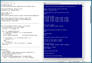 [Click on image for larger view.] Figure 1: Gaussian Process Regression in Action /figcaption>
After training, the model is applied to the training data and the test data. The model scores 97.50 percent accuracy (195 correct out of 200) on the training data, and 75.00 percent accuracy (30 correct out of 40) on the test data. The demo program defines a correct prediction as one that's within 10 percent of the true target value.
The demo concludes by predicting the target value of a new, previously unseen data item with predictor x values of (-0.5, 0.5, -0.5, 0.5, -0.5). The predicted y value is 0.0993 with a standard deviation of 0.0517.
This article assumes you have intermediate or better skill with a C-family programming language, but doesn't assume you know much about Gaussian process regression or the scikit library. The complete source code for the demo program is presented in this article and in the accompanying file download. The source code and data are also available online.
Installing the scikit Library
There are several ways to install the scikit library. I recommend installing the Anaconda Python distribution. Anaconda contains a core Python engine plus over 500 libraries that are (mostly) compatible with each other. I used Anaconda3-2022.10, which contains Python 3.9.13 and the scikit 1.0.2 version. The demo code runs on Windows 10 or 11.
Briefly, Anaconda / Python / scikit is installed using a Windows self-extracting executable file. The setup process is mostly straightforward and takes about 15 minutes following step-by-step instructions.
There are more up-to-date versions of Anaconda / Python / scikit library available. But because the Python ecosystem has hundreds of libraries, if you install the most recent versions of these libraries, you run a greater risk of library incompatibilities -- this is a major headache when working with Python.
The Data
The data is synthetic and was generated by a 5-10-1 neural network with random weights and biases. The point is that there is an underlying model that should be discoverable to some extent (as opposed to purely random data).
There are 200 training items and 40 test items. The structure of data looks like:
-0.1660   0.4406  -0.9998  -0.3953  -0.7065  0.1672
 0.0776  -0.1616   0.3704  -0.5911   0.7562  0.6022
-0.9452   0.3409  -0.1654   0.1174  -0.7192  0.2288
 0.9365  -0.3732   0.3846   0.7528   0.7892  0.0379
. . .
Each line of tab-delimited data has five predictor values followed by the target value to predict. The predictor values are all between -1.0 and +1.0 (corresponding to real data that has been normalized). The target values are all between 0.0 and 1.0.
Gaussian process regression was designed for problems with strictly numeric predictor variables. However, GPR can be used with categorical predictor variables by using one-hot encoding. For example, if the source data has a variable Color with possible values red, blue, green and yellow, then red can be encoded as 1000, blue = 0100, green = 0010 and yellow = 0001.
When using GPR you should normalize numeric predictor variables so that all values are roughly in the same range. This prevents variables with large magnitudes, such as annual income, from overwhelming variables with small values, such as college GPA.
Understanding Gaussian Process Regression
The mathematics of Gaussian process regression is complex. There are hundreds of web pages and hundreds of hours of video that attempt to explain GPR. The mere fact that there are so many resources available is an indication of how tricky the topic is.
There is no single best resource for GPR theory -- it all depends on a person's background and extent of understanding of topics including kernel functions, covariance matrices, multivariate Gaussian distributions, regularization, Bayesian mathematics and matrix operations. That said, it is possible to create effective GPR prediction models using the scikit library without having deep knowledge of the underlying theory.
A key concept of GPR is the idea of a kernel function. A kernel function accepts two vectors and computes a measure of similarity/dissimilarity. There are many different types of kernel functions and each type has several variations.
One of the most commonly used kernel functions is the radial basis function (RBF). The variation of RBF used by the scikit GaussianProcessRegressor module is rbf(x1, x2) = exp( -1 * ||x1 - x2||^2 / (2 * s^2) ) where x1 and x2 are vectors. The ||x1 - x2||^2 term is squared Euclidean distance between x1 and x2. The s term is the length scale and is a constant that must be specified.
Suppose x1 = (0.4, 0.8, 0.2) and x2 = (0.1, 0.6, 0.3) and s = 1.0. Then:
||x1 - x2||^2 = (0.4 - 0.1)^2 + (0.8 - 0.6)^2 + (0.2 - 0.3)^2
              = 0.09 + 0.04 + 0.01
              = 0.14
and therefore:
rbf(x1, x2) = exp( -1 * ||x1 - x2||^2 / (2 * s^2) )
            = exp( -1 * 0.14 / (2 * 1.0^2) )
            = exp(-0.07)
            = 0.9324
In addition to the RBF kernel function, the scikit GaussianProcessRegressor module supports the ConstantKernel, Matern, RationalQuadratic, ExpSineSquared and DotProduct kernel functions. The main challenge when using GPR is finding a good kernel function. There are few rules of thumb, and it's mostly a matter of trial and error guided by experience.
The Demo Program
The complete demo program is presented in Listing 1. Notepad is my code editor of choice but most of my colleagues prefer one of the many excellent IDEs that are available for Python. I indent my Python program using two spaces rather than the more common four spaces.
The program imports the NumPy library, which contains numeric array functionality, the pickle module used for saving a trained model, and the GaussianProcessRegressor module, which contains GPR functionality. Notice the name of the root scikit module is sklearn rather than scikit.
import numpy as np
import pickle
from sklearn.gaussian_process import GaussianProcessRegressor
In terms of Python style, I prefer to place all the import statements at the top of a program. An alternative is to place each import statement near its first usage.
Listing 1: Complete Demo Program
# synthetic_gpr.py
# scikit Gaussian process regression on synthetic data

# Anaconda3-2022.10  Python 3.9.13
# scikit 1.0.2  Windows 10/11

import numpy as np
import pickle
from sklearn.gaussian_process import GaussianProcessRegressor

from sklearn.gaussian_process.kernels import RBF
# RBF, ConstantKernel, Matern, RationalQuadratic,
# ExpSineSquared, DotProduct

# -----------------------------------------------------------

def accuracy(model, data_X, data_y, pct_close):
  # correct within pct of true target
  n_correct = 0; n_wrong = 0

  for i in range(len(data_X)):
    X = data_X[i].reshape(1, -1)  # one-item batch
    y = data_y[i]
    pred = model.predict(X)       # predicted target value

    if np.abs(pred - y) < np.abs(pct_close * y):
      n_correct += 1
    else:
      n_wrong += 1
  acc = (n_correct * 1.0) / (n_correct + n_wrong)
  return acc

# -----------------------------------------------------------

def main():
  # 0. prepare
  print("\nBegin scikit Gaussian process regression ")
  print("Predict synthetic data ")
  np.random.seed(1)
  np.set_printoptions(edgeitems=5, linewidth=100,
    sign=" ", formatter={'float': '{: 7.4f}'.format})

# -----------------------------------------------------------

  # 1. load data
  print("\nLoading 200 train and 40 test data for GPR ")
  train_file = ".\\Data\\synthetic_train.txt"
  train_X = np.loadtxt(train_file, delimiter="\t",
    usecols=(0,1,2,3,4),
    comments="#", dtype=np.float64)
  train_y = np.loadtxt(train_file, delimiter="\t",
    usecols=5, comments="#", dtype=np.float64)

  test_file = ".\\Data\\synthetic_test.txt"
  test_X = np.loadtxt(test_file, delimiter="\t",
    usecols=(0,1,2,3,4),
    comments="#", dtype=np.float64)
  test_y = np.loadtxt(test_file, delimiter="\t",
    usecols=5, comments="#", dtype=np.float64)
  print("Done ")

  print("\nFirst four X data: ")
  print(train_X[0:4][:])
  print(". . .")
  print("\nFirst four targets: ")
  print(train_y[0:4])
  print(". . .")

# -----------------------------------------------------------

  # 2. create and train GPR model
  print("\nCreating GPR model with RBF(1.0) kernel ")

  # GaussianProcessRegressor(kernel=None, *, alpha=1e-10,
  #  optimizer='fmin_l_bfgs_b', n_restarts_optimizer=0,
  #  normalize_y=False, copy_X_train=True, random_state=None)
  #
  # default: ConstantKernel(1.0, constant_value_bounds="fixed")
  #  * RBF(1.0, length_scale_bounds="fixed")
  # scikit-learn.org/stable/modules/gaussian_process.html

  krnl = RBF(length_scale=1.0, length_scale_bounds="fixed")
  gpr_model = GaussianProcessRegressor(kernel=krnl,
    normalize_y=False, random_state=1, alpha=0.001)
  print("Done ")

  print("\nTraining model ")
  gpr_model.fit(train_X, train_y)
  print("Done ")

# -----------------------------------------------------------

  # 3. compute model accuracy
  print("\nComputing accuracy (within 0.10 of true) ")
  acc_train = accuracy(gpr_model, train_X, train_y, 0.10)
  print("\nAccuracy on train data = %0.4f " % acc_train)
  acc_test = accuracy(gpr_model, test_X, test_y, 0.10)
  print("Accuracy on test data = %0.4f " % acc_test)

  # 4. use model to predict
  x = np.array([[-0.5, 0.5, -0.5, 0.5, -0.5]],
    dtype=np.float64)
  print("\nPredicting for x = ")
  print(x)
  (y_pred, std) = gpr_model.predict(x, return_std=True)
  print("\nPredicted y = %0.4f " % y_pred)
  print("std = %0.4f " % std)

  # 5. save model
  print("\nSaving trained GPR model ")
  fn = ".\\Models\\gpr_model.pkl"
  with open(fn,'wb') as f:
    pickle.dump(gpr_model, f)

  print("\nEnd GPR prediction ")

# -----------------------------------------------------------

if __name__ == "__main__":
  main()
All the program logic is contained in a main() function. The demo defines an accuracy() function that emphasizes clarity at the expense of efficiency. The demo begins by setting the NumPy random seed:
def main():
  # 0. prepare
  print("Begin scikit Gaussian process regression ")
  print("Predict synthetic data ")
  np.random.seed(1)
  np.set_printoptions(edgeitems=5, linewidth=100,
    sign=" ", formatter={'float': '{: 7.4f}'.format})
 . . .
Technically, setting the random seed value isn't necessary, but doing so helps you to get reproducible results in many situations where there are one or more random components. The GaussianProcessRegressor module can be instructed to try to programmatically optimize its kernel function parameters, and that code has a random component.
Loading the Training and Test Data
The demo program loads the training data into memory using these statements:
  # 1. load data
  print("Loading 200 train and 40 test data for GPR ")
  train_file = ".\\Data\\synthetic_train.txt"
  train_X = np.loadtxt(train_file, delimiter="\t",
    usecols=(0,1,2,3,4),
    comments="#", dtype=np.float64)  # 2-D
  train_y = np.loadtxt(train_file, delimiter="\t",
    usecols=5, comments="#", dtype=np.float64)  # 1-D
This code assumes the data files are stored in a directory named Data. There are many ways to load data into memory. I prefer using the NumPy library loadtxt() function, but a common alternative is the Pandas library read_csv() function.
The code reads training and test data using one call to loadtxt() for the predictor values and a second call to loadtxt() for the target values. An alternative approach is to read both predictor and target values into a matrix using a single call to loadtxt() and then split the matrix into a matrix of predictors and a vector of target values.
The 40-item test data is read into memory in the same way as the training data:
  test_file = ".\\Data\\synthetic_test.txt"
  test_X = np.loadtxt(test_file, delimiter="\t",
    usecols=(0,1,2,3,4),
    comments="#", dtype=np.float64)
  test_y = np.loadtxt(test_file, delimiter="\t",
    usecols=5, comments="#", dtype=np.float64)
  print("Done ")
The demo program prints the first four predictor items and the first four target values in the training data:
  print("First four X data: ")
  print(train_X[0:4][:])
  print(". . .")
  print("First four targets: ")
  print(train_y[0:4])
  print(". . .")
In a non-demo scenario you might want to display all the training data and all the test data to verify the data has been read properly.
Creating and Training the Gaussian Process Regression Model
Creating the Gaussian process regression model is simultaneously simple and complicated. The code is relatively short:
  # 2. create and train GPR model
  print("Creating GPR model with RBF(1.0) kernel ")
  krnl = RBF(length_scale=1.0, length_scale_bounds="fixed")
  gpr_model = GaussianProcessRegressor(kernel=krnl,
    normalize_y=False, random_state=1, alpha=0.001)
  print("Done ")
An RBF kernel with length scale = 1.0 is specified. The length_scale="fixed" instructs the module to not try to programmatically optimize the length scale parameter that has just been set to 1.0. In my experience, programmatically optimizing kernel parameter(s) usually leads to a worse model than fixing the parameter value(s).
The demo sets the GaussianProcessRegressor constructor random_state parameter to 1, but this has no effect because kernel parameter optimization is not being used. So, the random_state parameter could be dropped.
The alpha parameter controls regularization, which is an attempt to limit model overfitting when a model predicts training data well but predicts test data poorly. GPR is highly susceptible to model overfitting, so a good value for alpha is critical. Larger values of alpha reduce overfitting, but a too-large value can create a model with very poor accuracy.
After the GPR model has been created, training is almost too simple:
  print("Training model ")
  gpr_model.fit(train_X, train_y)
  print("Done ")
All of the decisions are made with the kernel and constructor parameters, so there's not much to think about. I usually explore GPR hyperparameters using a grid search. First, I define a root mean squared error function like so:
def root_mse(model, data_X, data_y):
  preds = model.predict(data_X)
  sum = np.sum((preds - data_y)**2)
  return np.sqrt(sum / len(data_y))
Then I set up candidate hyperparameter values, for example:
scales = [0.1, 0.5, 1.0, 1.5, 2.0]
alphas = [0.0, 0.0001, 0.001, 0.01, 0.1]
And then I examine the different combinations of hyperparameter values:
for s in scales:
  for a in alphas:
    krnl = RBF(length_scale=s, length_scale_bounds="fixed")
    gpr_model = GaussianProcessRegressor(kernel=krnl,
      normalize_y=False, random_state=1, alpha=a)
    gpr_model.fit(train_X, train_y)
    train_acc = accuracy(gpr_model, train_X, train_y, 0.10)
    train_rmse = root_mse(gpr_model, train_X, train_y)
    print("scale = %0.1f alpha = %0.4f |  acc = %0.4f \
      rmse = %0.4f " % (s, a, train_acc, train_rmse))
The idea is to find a set of hyperparameter values that balance root mean squared error -- which is a fine-grained measure of model goodness -- with accuracy, which is coarse but ultimately what you're interested in.
Evaluating the Trained Model
The demo computes the accuracy of the trained model like so:
  # 3. compute model accuracy
  print("Computing accuracy (within 0.10 of true) ")
  acc_train = accuracy(gpr_model, train_X, train_y, 0.10)
  print("Accuracy on train data = %0.4f " % acc_train)
  acc_test = accuracy(gpr_model, test_X, test_y, 0.10)
  print("Accuracy on test data = %0.4f " % acc_test)
For most scikit classifiers, the built-in score() function computes a simple accuracy, which is just the number of correct predictions divided by the total number of predictions. But for a GaussianProcessRegressor regression model, you must define what a correct prediction is and write a program-defined custom accuracy function. The accuracy() function in Listing 1 defines a correct prediction as one that is within a specified percentage of the true target value. The key statement is:
if np.abs(pred - y) < np.abs(pct_close * y):
  n_correct += 1
else:
  n_wrong += 1
The pred variable is the predicted value and the y is the known correct target value. In words, "if the difference between predicted and actual values is less than x percent of the actual target, then the prediction is correct."
Using and Saving the Trained Model
The demo uses the trained model like so:
  # 4. use model to predict
  x = np.array([[-0.5, 0.5, -0.5, 0.5, -0.5]],
    dtype=np.float64)
  print("Predicting for x = ")
  print(x)
  (y_pred, std) = gpr_model.predict(x, return_std=True)
  print("Predicted y = %0.4f " % y_pred)
  print("std = %0.4f " % std)
Because the GPR model was trained using normalized data, the X-input must be normalized in the same way; in other words, all predictors must be between -1 and +1. Notice the double square brackets on the X-input. The predict() method expects a matrix rather than a vector.
A significant characteristic of a GPR model is that it predicts a value but can also return a standard deviation, which is a measure of uncertainty. For the demo data, the predicted value for the dummy inputs is 0.0993 and the standard deviation is 0.0517. Therefore, the prediction could be stated as, "0.0993 plus or minus one standard deviation of 0.0517."
In most situations you will want to save the trained regression model so that it can be used by other programs. There are several ways to save a scikit model but using the pickle library ("pickle" means to preserve in ordinary English) is the simplest and most common. The demo code is:
  # 5. save model
  print("Saving trained GPR model ")
  fn = ".\\Models\\gpr_model.pkl"
  with open(fn,'wb') as f:
    pickle.dump(gpr_model, f)
This code assumes there is a subdirectory named Models. The saved model can be loaded into memory and used like this:
  # load and use model
  path = ".\\Models\\gpr_model.pkl"
  with open(path, 'rb') as f:
    loaded_model = pickle.load(f)
  X = (set some values for X)
  (y_pred, std) = loaded_model.predict(X)
A pickle file uses a proprietary binary format. An alternative is to write a custom save() function that saves model information as plain text. This is useful if a trained model is going to be consumed by a non-Python program.
Wrapping Up
Many of my colleagues shy away from using Gaussian process regression, mostly because the underlying mathematics are very complex. But when GPR works, it often works very well.
GPR is well-suited for relatively small datasets where the data is strictly numeric. Behind the scenes, GPR computes the inverse of a matrix with a size based on the number of training items. As mentioned earlier, GPR can handle categorical predictor variables by using one-hot encoding.
A regression technique that is closely related to Gaussian process regression is kernel ridge regression (KRR). KRR and GPR have different mathematical assumptions, but surprisingly end up with the same prediction equation. The GPR assumptions are more restrictive and so GPR can generate a metric (standard deviation / variance) of prediction uncertainty, but KRR can only produce a point prediction.