The Data Science Lab
Spectral Data Clustering from Scratch Using C#
Spectral clustering is quite complex, but it can reveal patterns in data that aren't revealed by other clustering techniques.
Data clustering is the process of grouping data items so that similar items are placed in the same cluster. There are several different clustering techniques and each technique has many variations. Common clustering techniques include k-means, Gaussian mixture model, density-based and spectral. This article explains how to implement one possible version of spectral clustering from scratch using the C# programming language.
Compared to other clustering techniques, spectral clustering is very complex from both a theoretical and implementation point of view. But spectral clustering can reveal patterns in data that aren't revealed by other clustering techniques. Spectral clustering is a meta-algorithm, meaning that there are dozens of variations.
The demo implementation uses a radial basis function (RBF) kernel to construct the affinity matrix, a normalized Laplacian matrix based on weights, embedding using eigenvectors via QR decomposition and k-means clustering. If you're not familiar with spectral clustering, this probably sounds confusing, but the meanings should become clear shortly.
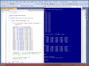 [Click on image for larger view.] Figure 1: Spectral Data Clustering in Action
A good way to see where this article is headed is to take a look at the screenshot of a demo program in Figure 1. For simplicity, the demo uses just N = 18 data items:
0.20, 0.20
0.20, 0.70
0.30, 0.90
. . .
0.80, 0.80
0.50, 0.90
Each data item is a vector with dim = 2 elements. The spectral clustering technique is designed for strictly numeric data.
The demo displays the first five rows and five columns of two of the key matrices that are computed by the spectral clustering algorithm. The 18-by-18 affinity matrix holds values that are measures of the similarity between data items. The 18-by-18 Laplacian matrix can be loosely thought of as a graph representation of the data items.
After clustering with k = 2, the resulting clustering is: (0, 0, 0, 1, 1, 1, 0, 0, 0, 0, 0, 0, 0, 0, 0, 0, 0, 0). This means data items [3], [4], [5] are assigned to cluster 1, and the other 15 data items are assigned to cluster 0. Cluster IDs are arbitrary so a clustering of (0, 0, 1, 0) is equivalent to a clustering of (1, 1, 0, 1). Cluster IDs are sometimes called labels.
The data, before and after spectral clustering, is shown in Figure 2. Notice that there is no inherent best clustering of data. The results look reasonable but many other clusterings are possible.
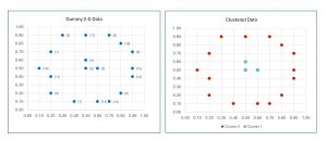 [Click on image for larger view.] Figure 2: Demo Data Before and After Spectral Clustering
This article assumes you have intermediate or better programming skill but doesn't assume you know anything about spectral clustering. The demo is implemented using C# but you should be able to refactor the demo code to another C-family language if you wish.
The source code for the demo program is too long to be presented in this article. The complete code is available in the accompanying file download and is also available online.
The Demo Program
I used Visual Studio 2022 (Community Free Edition) for the demo program. I created a new C# console application and checked the "Place solution and project in the same directory" option. I specified .NET version 6.0. I named the project SpectralClustering. I checked the "Do not use top-level statements" option to avoid the program entry point shortcut syntax.
The demo has no significant .NET dependencies and any relatively recent version of Visual Studio with .NET (Core) or the older .NET Framework will work fine. You can also use the Visual Studio Code program if you like.
After the template code loaded into the editor, I right-clicked on file Program.cs in the Solution Explorer window and renamed the file to the slightly more descriptive SpectralClusteringProgram.cs. I allowed Visual Studio to automatically rename class Program.
The Main() method starts by loading the 18-item dummy data into memory as an array-of-arrays style matrix:
double[][] X = new double[18][];
X[0] = new double[] { 0.20, 0.20 };
X[1] = new double[] { 0.20, 0.70 };
. . .
X[17] = new double[] { 0.50, 0.90 };
For simplicity, the data is hard-coded. In a non-demo scenario you'll probably want to load the data from a text file using a program-defined helper function:
string fn = "..\\..\\..\\Data\\dummy_data_18.txt";
double[][] X = MatLoad(fn, new int[] { 0, 1 },
  ',', "#");
Console.WriteLine("Data: ");
MatShow(X, 2, 6);  // helper
The arguments to MatLoad() mean fetch columns 0 and 1 of the comma-separated data, where a "#" character indicates a comment line.
When using spectral clustering, the data should be normalized so that all columns have roughly the same magnitude so that columns with large magnitudes don't dominate the clustering.
The spectral clustering object is created and used like so:
int k = 2;
double gamma = 50.0;  // RBF affinity
Spectral sp = new Spectral(k, gamma);
int[] clustering = sp.Cluster(X);
Console.WriteLine("spectral clustering: ");
VecShow(clustering, 2);  // helper
The number of clusters, k, must be specified. Loosely speaking, the gamma argument controls how close two data items must be for them to be considered neighbors. Spectral clustering results are highly sensitive to the value of gamma, and a good value must be determined by trial and error.
Understanding Spectral Clustering
Spectral clustering is either simple or extremely complex depending on your point of view. Expressed in high-level pseudo-code, there are five main steps:
    read source data into memory as a matrix X
    use X to compute an affinity matrix A
    use A to compute a Laplacian matrix L
    use L to compute an eigenvector embedding matrix E
    perform standard clustering on E
Each of the five steps is a significant, but manageable, problem. Briefly, the source data is transformed into an alternative representation and then standard data clustering is performed on the transformed data. The demo code (without calls to the MatShow() function to display the affinity and Laplacian matrices) that corresponds to the pseudo-code is:
public int[] Cluster(double[][] X)
{
  double[][] A = this.MakeAffinityRBF(X);  // RBF
  double[][] L = this.MakeLaplacian(A);    // normalized
  double[][] E = this.MakeEmbedding(L);    // eigenvectors
  int[] result = this.ProcessEmbedding(E); // k-means
  return result;
}
So, the keys to understanding the demo implementation of spectral clustering are understanding how to compute RBF and affinity matrices, how to compute Laplacian matrices, how to compute eigenvector embeddings and how to perform k-means clustering.
Of the spectral clustering sub-problems, computing the eigenvectors from the Laplacian matrix is blisteringly complex. Wikipedia lists 14 different algorithms for computing eigenvectors, and each of these has several variations. The demo program uses the QR algorithm variation to compute eigenvectors, and the Householder algorithm variation to compute QR. Yikes!
The RBF Kernel Function and the Affinity Matrix
A radial basis function computes a number which is a measure of the similarity between two vectors. If two vectors are the same, RBF is 1.0 (maximum similarity). As two vectors increase in difference, RBF approaches, but never quite reaches 0.0. The demo implementation is:
private static double MyRBF(double[] v1, double[] v2,
  double gamma)
{
  int dim = v1.Length;
  double sum = 0.0;
  for (int i = 0; i < dim; ++i)
    sum += (v1[i] - v2[i]) * (v1[i] - v2[i]);
  return Math.Exp(-gamma * sum);
}
The gamma parameter affects the rate at which the RBF value approaches zero as vectors v1 and v2 increase in difference.
An affinity matrix A holds the RBF values for each data item compared to every other data item. The value of A[i][j] is the RBF of data item [i] and data item [j]. The values on the diagonal of an affinity matrix are 1 (the RBF of an item with itself). The values off the diagonal will be symmetric because RBF(v1, v2) = RBF(v2, v1). For the demo data, because there are 18 data items, the affinity matrix will be 18-by-18.
An affinity matrix is sometimes called a similarity matrix, but this isn't entirely accurate. Alternative forms of spectral clustering use an affinity matrix where the values are 1 if two vectors are close (within a threshold value) or 0 if two vectors aren't close.
There are dozens of RBF functions. The demo uses a version that has several different names such as squared-exponential kernel and Gaussian kernel. But the version of RBF function used in the demo is very common and so it's often referred to as just the RBF kernel.
The Laplacian Matrix
There are several of types of Laplacian matrices. Most have the general form of L = D - A where D is a degree matrix and A is an adjacency matrix. For the special case of spectral clustering, A is the affinity matrix, and D is a matrix where the diagonal values are the row sums of A, and the off-diagonal values are zero.
The demo implementation is:
private double[][] MakeLaplacian(double[][] A)
{
  int n = A.Length;
  double[][] D = MatMake(n, n);  // degree matrix
  for (int i = 0; i < n; ++i) {
    double rowSum = 0.0;
    for (int j = 0; j < n; ++j)
      rowSum += A[i][j];
    D[i][i] = rowSum;
  }
  double[][] result = MatDifference(D, A);  // D-A
  return this.NormalizeLaplacian(result);
}
The MatMake() and MatDifference() functions are program-defined helpers. Because the only values that need to be computed are the diagonal values, using MatDifference() performs unnecessary calculations. But using MatDifference() is a cleaner approach in my opinion.
The resulting Laplacian matrix will have positive values on the diagonal, negative values off-diagonal and is called an unnormalized Laplacian. There are several ways to normalize a Laplacian matrix, typically by coercing the values on the diagonal to be 1. In a spectral clustering context with normalized data and an RBF affinity matrix, the Laplacian matrix values all have relatively small magnitudes and so Laplacian normalization is often not needed. The demo code applies a NormalizeLaplacian() function to normalize the Laplacian matrix.
The Eigenvector Embedding Matrix
If you have an n-by-n size matrix, it is possible to compute n eigenvalues (scalar values like 1.234) and n associated eigenvectors, each with n values. The eigenvalues and eigenvectors are paired with each other. You can think of the eigenvalue-eigenvector pairs as abstract characteristics of the source matrix. In mathematics, the set of the eigenvalues of a matrix is called the spectrum of the matrix, which is why spectral clustering is named as it is.
In spectral clustering, the eigenvalues and eigenvectors are computed from the Laplacian matrix. Computing eigenvalues and eigenvectors is one of the most difficult problems in numerical programming. There are several algorithms. The demo uses what is called the QR algorithm.
The C# language doesn't have a built-in function to compute eigenvalues and eigenvectors so it's necessary to implement one from scratch. After the eigenvalues and eigenvectors are computed from the Laplacian matrix, the k smallest eigenvalues are found and the associated k eigenvectors are extracted. This step is the key magic behind spectral clustering and the math theory is very deep.
The demo method that computes the eigenvalues and eigenvectors, and then extracts the k eigenvectors associated with the k smallest eigenvalues is:
private double[][] MakeEmbedding(double[][] L)
{
  double[] eigVals; double[][] eigVecs;
  EigenQR(L, out eigVals, out eigVecs); // QR algorithm
  int[] allIndices = ArgSort(eigVals);
  int[] indices = new int[this.k]; // small eigenvecs
  for (int i = 0; i < this.k; ++i)
    indices[i] = allIndices[i];
  double[][] extracted = MatExtractCols(eigVecs, indices);
  return extracted;
}
The program-defined EigenQR() function is the most complicated part of the spectral clustering demo program. Implementing EigenQR() and its helper functions requires over 150 lines of code. But you can think of the function as a black box because you won't have to modify it for normal data clustering scenarios.
Computing eigenvalues and eigenvectors is time-consuming because it is O(n^3). Therefore, spectral clustering is not well-suited for very large datasets.
Clustering the Embedding
At this point, the 18-by-2 source data has been transformed into an 18-by-k embedding matrix of k eigenvectors (the columns). The last step in spectral clustering is to apply a standard clustering technique to the embedded data, which indirectly clusters the source data.
In practice, spectral clustering usually uses basic k-means clustering. This might seem a bit odd -- after jumping through all kinds of hoops, spectral clustering ends up applying the simplest form of clustering. The key idea is that spectral clustering transforms source data into a clever representation that allows k-means to find interesting patterns that wouldn't be found if k-means is applied directly to the source data.
The demo method code is:
private int[] ProcessEmbedding(double[][] E)
{
  KMeans km = new KMeans(E, this.k);
  int[] clustering = km.Cluster();
  return clustering;
}
Almost too simple. The demo program defines a nested KMeans class inside the top-level Spectral class. An alternative design is to define the KMeans class externally to the Spectral class.
Wrapping Up
The ideas behind spectral clustering are based on graph theory and were mostly introduced in the 1960s. But using the ideas for machine learning data clustering is relatively new -- dating from roughly 2001. Spectral clustering is sometimes applied to image data when the technique is known as segmentation-based object categorization.
I suspect that there is one main reason why spectral data clustering is not used very often. The technique is based on deep mathematics and people who don't have a basic familiarity with similarity metrics, affinity matrices, Laplacian matrices, eigenvalues and eigenvectors, may shy away from using spectral clustering. This is especially true when there are much simpler clustering techniques available, notably k-means and DBSCAN, combined with the fact that there is no objective measure of how good any data clustering result is.