The Data Science Lab
Principal Component Analysis (PCA) from Scratch Using the Classical Technique with C#
Transforming a dataset into one with fewer columns is more complicated than it might seem, explains Dr. James McCaffrey of Microsoft Research in this full-code, step-by-step machine learning tutorial.
Principal component analysis (PCA) is a classical machine learning technique. The goal of PCA is to transform a dataset into one with fewer columns. This is called dimensionality reduction. The transformed data can be used for visualization or as the basis for prediction using ML techniques that can't deal with a large number of predictor columns.
There are two main techniques to implement PCA. The first technique computes eigenvalues and eigenvectors from a covariance matrix derived from the source data. The second PCA technique sidesteps the covariance matrix and computes a singular value decomposition (SVD) of the source data. Both techniques give the same results, subject to very small differences.
This article presents a from-scratch C# implementation of the first technique: compute eigenvalues and eigenvectors from the covariance matrix. If you're not familiar with PCA, most of the terminology -- covariance matrix, eigenvalues and eigenvectors and so on -- sounds quite mysterious. But the ideas will become clear shortly.
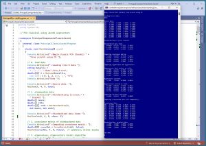 [Click on image for larger view.] Figure 1: PCA Using the Classical Technique with C# in Action
A good way to see where this article is headed is to take a look at the screenshot of a demo program in Figure 1.
For simplicity, the demo uses just nine data items:
[0]   5.1000   3.5000   1.4000   0.2000
[1]   4.9000   3.1000   1.5000   0.1000
[2]   5.1000   3.8000   1.5000   0.3000
[3]   7.0000   3.2000   4.7000   1.4000
[4]   5.0000   2.0000   3.5000   1.0000
[5]   5.9000   3.2000   4.8000   1.8000
[6]   6.3000   3.3000   6.0000   2.5000
[7]   6.5000   3.2000   5.1000   2.0000
[8]   6.9000   3.2000   5.7000   2.3000
The nine data items are one-based items 1, 10, 20, 51, 61, 71, 101, 111 and 121 of the 150-item Iris dataset. Each line represents an iris flower. The four columns are sepal length, sepal width, petal length and petal width (a sepal is a green leaf-like structure). Because there are four columns, the data is said to have dimension = 4.
The leading index values in brackets are not part of the data. Each data item is one of three species: 0 = setosa, 1 = versicolor 2 = virginica. The first three items are setosa, the second three items are versicolor and the last three items are virginica. The species labels were removed because they're not used for PCA dimensionality reduction.
PCA is intended for use with strictly numeric data. Mathematically, the technique works with Boolean variables (0-1 encoded) and for one-hot encoded categorical data. Conceptually, however, applying PCA to non-numeric data is questionable, and there is very little research on the topic.
The demo program applies z-score normalization to the source data. Then a 4-by-4 covariance matrix is computed from the normalized data. Next, four eigenvalues and four eigenvectors are computed from the covariance matrix (using the Jacobi algorithm). Next, the demo uses the eigenvectors to compute transformed data:
[0]  -2.0787   0.6736  -0.0425   0.0435
[1]  -2.2108  -0.2266  -0.1065  -0.0212
[2]  -2.0071   1.2920   0.1883   0.0025
[3]   1.1557   0.3503  -0.9194  -0.0785
[4]  -0.7678  -2.6702   0.0074   0.0115
[5]   0.7029  -0.0028   0.4066  -0.0736
[6]   1.8359   0.2191   0.6407  -0.0424
[7]   1.3476   0.1482  -0.0201   0.0621
[8]   2.0224   0.2163  -0.1545   0.0960
At this point, in a non-demo scenario, you could extract the first two or first three of the columns of the transformed data to use as a surrogate for the source data. For example, if you used the first two columns, you could graph the data with the first column acting as x-values and the second column acting as y-values.
The demo program concludes by programmatically reconstructing the source data from the transformed data. The idea is to verify the PCA worked correctly and also to illustrate that the transformed data contains all of the information in the source data.
This article assumes you have intermediate or better programming skill but doesn't assume you know anything about principal component analysis. The demo is implemented using C#, but you should be able to refactor the demo code to another C-family language if you wish. All normal error checking has been removed to keep the main ideas as clear as possible.
The source code for the demo program is too long to be presented in its entirety in this article. The complete code is available in the accompanying file download, and is also available online.
Understanding Principal Component Analysis
The best way to understand PCA is to take a closer look at the demo program. The demo has eight steps:
- load data into memory
- normalize the data
- compute a covariance matrix from the normalized data
- compute eigenvalues and eigenvectors from covariance matrix
- sort the eigenvectors based on eigenvalues
- compute variance explained by each eigenvector
- use eigenvectors to compute transformed data
- verify by reconstructing source data
The demo loads the source data using a helper MatLoad() function:
Console.WriteLine("Loading Iris-9 data ");
string dataFile = "..\\..\\..\\Data\\iris_9.txt";
double[][] X = MatLoad(dataFile, new int[] { 0, 1, 2, 3 },
  ',', "#");
Console.WriteLine("Source data: ");
MatShow(X, 4, 9, true);
The arguments to MatLoad() mean fetch columns 0,1,2,3 of the comma-separated data, where a "#" character indicates a comment line. The arguments to MatShow() mean display using four decimals, with a field width of nine per element, and display indices.
Normalizing the Data
Each column of the data is normalized using these statements:
Console.WriteLine("Standardizing (z-score, biased) ");
double[] means;
double[] stds;
double[][] stdX = MatStandardize(X, out means, out stds);
Console.WriteLine("Standardized data items ");
MatShow(stdX, 4, 9, nRows: 3);
The four means and standard deviations for each column are saved because they are needed to reconstruct the original source data. The terms standardization and normalization are technically different but are often used interchangeably. Standardization is a specific type of normalization (z-score). PCA documentation tends to use the term standardization, but I sometimes use the more general term normalization.
Each value is normalized using the formula x' = (x - u) / s, where x' is the normalized value, x is the original value, u is the column mean and s is the column biased standard deviation (divide sum of squares by n rather than n-1 where n is the number of values in the column).
For example, suppose a column of some data has just n = 3 values: (4, 15, 8). The mean of the column is (4 + 15 + 8) / 3 = 9.0. The biased standard deviation of the column is sqrt( ((4 - 9.0)^2 + (15 - 9.0)^2 + (8 - 9.0)^2) / n) ) = sqrt( (25.0 + 36.0 + 1.0) / 3 ) = sqrt(62.0 / 3) = 4.55.
The normalized values for (4, 15, 8) are:
 4: (4 - 9.0)  / 4.55 = -1.10
15: (15 - 9.0) / 4.55 =  1.32
 8: (8 - 9.0)  / 4.55 = -0.22
Normalized values that are negative are less than the column mean, and normalized values that are positive are greater than the mean. For the demo data, the normalized data is:
 -0.9410   0.7255  -1.3515  -1.2410
 -1.1901  -0.1451  -1.2952  -1.3550
 -0.9410   1.3784  -1.2952  -1.1270
  1.4253   0.0725   0.5068   0.1266
 -1.0655  -2.5392  -0.1689  -0.3292
  0.0554   0.0725   0.5631   0.5825
  0.5535   0.2902   1.2389   1.3803
  0.8026   0.0725   0.7321   0.8105
  1.3008   0.0725   1.0700   1.1524
After normalization, each value in a column will typically be between -3.0 and +3.0. Normalized values that are less than -6.0 or greater than +6.0 are extreme and should be investigated. The idea behind normalization is to prevent columns with large values (such as employee annual salaries) from overwhelming columns with small values (such as employee age).
Computing the Covariance Matrix
The covariance matrix of the normalized source data is computed like so:
Console.WriteLine("Computing covariance matrix: ");
double[][] covarMat = CovarMatrix(stdX, false);
MatShow(covarMat, 4, 9, false);
The "false" argument in the call to CovarMatrix() means to treat the data as if it is organized so that each variable (sepal length, sepal width, petal length and petal width) is in a column. A "true" argument means the data variables are organized as rows. I use this interface to match that of the Python numpy.cov() library function.
The covariance of two vectors is a measure of the joint variability of the vectors. For example, if v1 = [4, 9, 8] and v2 = [6, 8, 1], then covariance(v1, v2) = -0.50. Loosely speaking, the closer the covariance is to 0, the less associated the two vectors are. The larger the covariance, the greater the association. The sign of the covariance indicates the direction of the association. There's no upper limit on the magnitude of a covariance because it will increase as the number of elements in the vectors increases. See my article, "Computing the Covariance of Two Vectors Using C#", for a worked example.
A covariance matrix stores the covariance between all pairs of columns in the normalized data. For example, cell [0][3] of the covariance matrix holds the covariance between column 0 and column 3. For the demo data, the covariance matrix is:
 1.1250   0.1649   0.9538   0.9147
 0.1649   1.1250  -0.1976  -0.1034
 0.9538  -0.1976   1.1250   1.1095
 0.9147  -0.1034   1.1095   1.1250
Notice that the covariance matrix is symmetric because covariance(x, y) = covariance(y, x). The values on the diagonal of the covariance matrix are all the same (1.1250) due to the z-score normalization.
Computing the Eigenvalues and Eigenvectors
The eigenvalues and eigenvectors of the covariance matrix are computed using this code:
Console.WriteLine("Computing eigenvalues and eigenvectors ");
double[] eigenVals;
double[][] eigenVecs;
Eigen(covarMat, out eigenVals, out eigenVecs);
Console.WriteLine("Eigenvectors (not sorted, as cols): ");
MatShow(eigenVecs, 4, 9, false);
For the demo data that has dim = 4, the covariance matrix of the normalized data has shape 4-by-4. There are four eigenvalues (single values like 1.234) and four eigenvectors, each with four values. The eigenvalues and eigenvectors are paired.
For the demo data, the four eigenvectors (as columns) are:
  0.5498   0.2395  -0.7823   0.1683
 -0.0438   0.9637   0.2420  -0.1035
  0.5939  -0.1102   0.2188  -0.7663
  0.5857  -0.0410   0.5306   0.6113
The program-defined Eigen() function returns the eigenvectors as columns, so the first eigenvector is (0.5498, -0.0438, 0.5939, 0.5857). The associated eigenvector is 3.1167. For PCA it doesn't help to overthink the deep mathematics of eigenvalues and eigenvectors. You can think of eigenvalues and eigenvectors as a kind of factorization of a matrix that captures all the information in the matrix in a sequential way.
Computing eigenvalues and eigenvectors is one of the most difficult problems in numerical programming. Because a covariance matrix is mathematically symmetric positive semidefinite (think "relatively simple structure"), it is possible to use a technique called the Jacobi algorithm to find the eigenvalues and eigenvectors. The majority of the demo code is the Eigen() function and its helpers.
Eigenvectors from a matrix are not unique in the sense that the sign is arbitrary. For example, an eigenvector (0.20, -0.50, 0.30) is equivalent to (-0.20, 0.50, -0.30). The eigenvector sign issue does not affect PCA.
Sorting the Eigenvalues and Eigenvectors
The next step in PCA is to sort the eigenvalues and their associated eigenvectors from largest to smallest. Some library eigen() functions return eigenvalues and eigenvectors already sorted, and some eigen() functions do not. The demo program assumes that the eigenvalues and eigenvectors are not necessarily sorted.
First, the four eigenvalues are sorted in a way that saves the ordering so that the paired eigenvectors can be sorted in the same order:
int[] idxs = ArgSort(eigenVals);  // to sort evecs
Array.Reverse(idxs);  // used later
Array.Sort(eigenVals);
Array.Reverse(eigenVals);
Console.WriteLine("Eigenvalues (sorted): ");
VecShow(eigenVals, 4, 9);
For the demo data, the sorted eigenvalues are (3.1167, 1.1930, 0.1868, 0.0036). The program-defined ArgSort() function doesn't sort but returns the order in which to sort from smallest to largest. The eigenvalues are sorted from smallest to largest using the built-in Array.Sort() function and then reversed to largest to smallest using the built-in Array.Reverse() function.
The eigenvectors are sorted using these statements:
eigenVecs = MatExtractCols(eigenVecs, idxs); // sort
eigenVecs = MatTranspose(eigenVecs);  // as rows
Console.WriteLine("Eigenvectors (sorted as rows):");
MatShow(eigenVecs, 4, 9, false);
The MatExtractCols() function pulls out each column in the eigenvectors, ordered by the idxs array, which holds the order in which to sort from largest to smallest. The now-sorted eigenvectors are converted from columns to rows using the MatTranspose() function only because that makes them a bit easier to read. The eigenvectors will have to be converted back to columns later. The point is that when you're looking at PCA documentation or working with PCA code, it's important to keep track of whether the eigenvectors are stored as columns (usually) or rows (sometimes).
Note: By pure coincidence, the Eigen() function for the nine-item demo data returns eigenvalues and eigenvectors that are already sorted. In most cases you must explicitly sort the eigenvalues and eigenvectors as demonstrated.
Computing the Variance Explained
The variance explained by each of the four eigenvalue-eigenvector pairs is computed from the sorted eigenvalues:
Console.WriteLine("Computing variance explained: ");
double[] varExplained = VarExplained(eigenVals);
VecShow(varExplained, 4, 9);
For the demo data, the sum of the sorted eigenvalues is 3.1167 + 1.1930 + 0.1868 + 0.0036 = 4.5000. The variance explained values are:
3.1167 / 4.5000 = 0.6926
1.1930 / 4.5000 = 0.2651
0.1868 / 4.5000 = 0.0415
0.0036 / 4.5000 = 0.0008
                  ------
                  1.0000
Loosely speaking, this means that the first eigenvector captures 69.26 percent of the information in the source data. The first two eigenvectors capture 0.6926 + 0.2651 = 95.77 percent of the information. The first three eigenvectors capture 0.6926 + 0.2651 + 0.0415 = 99.92 percent of the information. All four eigenvectors capture 100 percent of the information.
Computing the Transformed Data
After computing and sorting the eigenvalues and eigenvectors from the covariance matrix of the normalized data, the next step in PCA is to use the sorted eigenvectors to compute the transformed data:
Console.WriteLine("Computing transformed data (all components): ");
double[][] transformed = MatProduct(stdX, MatTranspose(eigenVecs));
Console.WriteLine("Transformed data: ");
MatShow(transformed, 4, 9, true);
The transformed data is the matrix product of the normalized data and the eigenvectors. Because the eigenvectors were converted to rows for easier viewing, they must be passed as columns using the MatTranspose() function.
The transformed data is:
[0]  -2.0787   0.6736  -0.0425   0.0435
[1]  -2.2108  -0.2266  -0.1065  -0.0212
[2]  -2.0071   1.2920   0.1883   0.0025
[3]   1.1557   0.3503  -0.9194  -0.0785
[4]  -0.7678  -2.6702   0.0074   0.0115
[5]   0.7029  -0.0028   0.4066  -0.0736
[6]   1.8359   0.2191   0.6407  -0.0424
[7]   1.3476   0.1482  -0.0201   0.0621
[8]   2.0224   0.2163  -0.1545   0.0960
The demo program concludes by reconstructing the original source data from the transformed data. First the normalized data is reconstructed like so:
Console.WriteLine("Reconstructing original data: ");
double[][] reconstructed = MatProduct(transformed, eigenVecs);
Notice that reconstruction uses eigenvectors as rows rather than columns. Once again, the eigenvectors columns-vs-rows issue can be tricky when working with PCA. Next, the original source data is recovered by multiplying by the standard deviations that were used to normalize the data, and then adding the means that were used:
for (int i = 0; i < reconstructed.Length; ++i)
  for (int j = 0; j < reconstructed[0].Length; ++j)
    reconstructed[i][j] = (reconstructed[i][j] * stds[j]) + means[j];
MatShow(reconstructed, 4, 9, 3);
Reconstructing the original source data from the transformed data is a good way to check that nothing has gone wrong with the PCA.
Wrapping Up
Principal component analysis can be used in several ways. One of the most common is to create a graph of data that has more than two columns. For the Iris data with four columns, there's no easy way to create a graph. But by applying PCA and then using the first of two transformed columns as the x-value and the second column as the y-value, a graph clearly reveals that species setosa items are quite different from the somewhat similar versicolor and virginica items.
Another way to use PCA is for anomaly detection. The idea is to use the first n columns of the transformed data, where the n columns capture roughly 60-80 percent of the variability, to approximately reconstruct the original source data. Data items that don't reconstruct accurately are anomalous in some way and should be investigated.