The Data Science Lab
Data Clustering Using a Self-Organizing Map (SOM) with C#
Dr. James McCaffrey of Microsoft Research presents a full-code, step-by-step tutorial on technique for visualizing and clustering data.
A self-organizing map (SOM) is a data structure that can be used for visualizing and clustering data. This article presents a from-scratch C# implementation of a SOM for data clustering.
Data clustering is the process of grouping similar data items into clusters. Based on my experience, the two most common data clustering techniques are k-means clustering and DBSCAN ("density based spatial clustering of applications with noise") clustering. Other clustering techniques include Gaussian mixture model clustering, spectral clustering and SOM clustering.
Compared to other techniques, SOM clustering produces a clustering where the clusters are constructed so that data item assigned to clusters with similar IDs are closer to each other than those in clusters with dissimilar cluster IDs. This provides additional information. For example, suppose you set k = 5 and so each data item falls into one of clusters (0, 1, 2, 3, 4). Data items in clusters 0 and 1 are closer to each other than data items in clusters 0 and 3.
Self-organizing maps can be used for several purposes other than clustering. A standard, non-clustering SOM usually creates a square matrix, such as 4-by-4, called the map. For a clustering SOM, even though you could create a square n-by-n matrix map, it usually makes more sense to create a 1-by-k matrix/vector map.
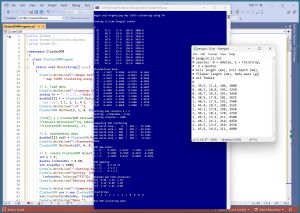 [Click on image for larger view.] Figure 1: SOM Data Clustering in Action
A good way to see where this article is headed is to take a look at the screenshot of a demo program in Figure 1. The demo starts by loading a small 12-item subset of the Penguin Dataset. Each item represents a penguin. The four columns are bill length, bill depth, flipper length and body mass. For simplicity, the data items are artificially ordered so that the first four items belong to one cluster, the second four items belong to a second cluster and the last four items belong to a third cluster.
Next, the data is z-score standardized (also called normalized) so that all column values are between -3 and +3. When using SOM clustering, in most scenarios the source data should be normalized.
The number of clusters is set to k = 3. The 1-by-3 SOM map is created using an iterative process with max steps = 1000 and max learning rate = 0.50. The resulting clustering assigns data items [0] to [3] to cluster 2, data items [4] to [7] are assigned to cluster 1, and data items [8] to [11] are assigned to cluster 0.
A post-clustering analysis of the results show that the data items in clusters 2 and 1, and in clusters 1 and 0, are closer together than the data items in clusters 2 and 0, as expected.
This article assumes you have intermediate or better programming skill but doesn't assume you know anything about SOM clustering. The demo is implemented using C#, but you should be able to refactor the demo code to another C-family language if you wish.
The source code for the demo program is a bit too long to be presented in its entirety in this article. The complete code is available in the accompanying file download, and is also available online. All normal error checking has been removed to keep the main ideas as clear as possible.
The Penguin Dataset
The demo program uses a small 12-item subset of the Penguin Dataset. The raw data is:
# penguin_12.txt
0, 39.5, 17.4, 186, 3800
0, 40.3, 18.0, 195, 3250
0, 36.7, 19.3, 193, 3450
0, 38.9, 17.8, 181, 3625
1, 46.5, 17.9, 192, 3500
1, 45.4, 18.7, 188, 3525
1, 45.2, 17.8, 198, 3950
1, 46.1, 18.2, 178, 3250
2, 46.1, 13.2, 211, 4500
2, 48.7, 14.1, 210, 4450
2, 46.5, 13.5, 210, 4550
2, 45.4, 14.6, 211, 4800
Each line represents one of three species of penguin. The fields are species (0 = Adelie, 1 = Chinstrap, 2 = Gentoo), bill length (mm), bill depth (mm), flipper length (mm) and body mass (g). The full Penguin Dataset has 333 valid (no NA values) items, and additional columns such as sex and year measured. The 12 demo data items all represent female penguins because SOM clustering, like most clustering techniques, is not designed to handle Boolean or categorical data.
I saved the 12-item data as penguin_12.txt in a directory named Data located in the project root directory. Because the raw data is artificially clustered by species, the SOM clustering results can be easily evaluated. In most non-demo data clustering scenarios, you don't know how many clusters there are, or how the data is clustered.
Standardizing the Data
The demo SOM implementation measures the distance between data items using Euclidean distance. Therefore, the source data must be normalized so that all columns have approximately the same magnitude. This prevents columns with large magnitudes, such as body mass, from overwhelming columns with small magnitudes.
The demo program uses z-score standardization. Technically, standardization is a specific type of normalization, but the terms standardization and normalization are often used interchangeably. To standardize a column, the mean and standard deviation of the column is computed, then the normalized values are x' = (x - u) / sd where x is the source data value, x' is the standardized value, u is the column mean, and sd is the column standard deviation.
For example, suppose a column of a dataset has just three values: 4, 15, 8. The mean of the column is (4 + 15 + 8) / 3 = 9.0. The standard deviation of the column is sqrt( (4 - 9.0)^2 + (15 - 9.0)^2 + (8 - 9)^2 ) = 4.5. The standardized values are:
 4: ( 4 - 9.0) / 4.5 = -1.11
15: (15 - 9.0) / 4.5 =  1.33
 8: ( 8 - 9.0) / 4.5 = -0.22
Standardized values will usually be between -3 and +3. Standardized values outside that range are extreme and should be investigated. Standardized values that are positive are greater than the column mean, and standardized values that are negative are less than the column mean.
The standardized demo data is:
-1.1657   0.3300  -0.8774  -0.1661
-0.9475   0.6163  -0.0943  -1.2103
-1.9291   1.2366  -0.2683  -0.8306
-1.3293   0.5209  -1.3125  -0.4984
 0.7430   0.5686  -0.3553  -0.7357
 0.4431   0.9503  -0.7034  -0.6882
 0.3886   0.5209   0.1668   0.1187
 0.6340   0.7117  -1.5735  -1.2103
 0.6340  -1.6740   1.2980   1.1628
 1.3429  -1.2445   1.2109   1.0679
 0.7430  -1.5308   1.2109   1.2578
 0.4431  -1.0060   1.2980   1.7324
An alternative to z-score standardization is divide-by-constant normalization. For example, you could divide the four columns of the source data by (50, 20, 200, 5000) respectively so that most normalized values are between 0 and 1. Another alternative to z-score standardization is min-max normalization. To the best of my knowledge, there is no research evidence to suggest that one normalization technique is better than others for SOM data clustering.
Understanding the SOM Map
The heart of SOM clustering is a 1-by-k matrix called the map. Each map cell (also called a node) holds a vector that is representative of the data items assigned to each cluster. The constructed SOM map nodes for the standardized demo data are:
k = 0:  0.8296  -1.4315   1.2489   1.2322
k = 1:  0.5188   0.7038  -0.4929  -0.5406
k = 2: -1.3109   0.6217  -0.6869  -0.6074
Data items that are closest to (0.8296, -1.4315, 1.2489, 1.2322) are assigned to cluster 0, data items closest to (0.5188, 0.7038, -0.4929, -0.5406) are assigned to cluster 1, and data items closest to (-1.3109, 0.6217, -0.6869, -0.6074) are assigned to cluster 2. For example, standardized data item [3] = (-1.3293, 0.5209, -1.3125, -0.4984) is clearly closest to map cell (-1.3109, 0.6217, -0.6869, -0.6074) and so data item [3] is assigned to cluster 2.
There are several variations of the SOM map construction algorithm. The demo program is based on the algorithm described in the Wikipedia article on self-organizing maps. The algorithm, expressed in very high-level pseudo-code, is:
    set max_steps
    set max_learn_rate
    init map cells to random vectors
    loop max_steps times
      pick a random data item
      find closest map cell vector ("BMU")
      update each close map cell vector
       using curr learn rate and
       curr Manhattan range
      end-update
      decrease curr learn_rate
      decrease curr Manhattan range
    end-loop
In the main processing loop, only map cell vectors that are close to the BMU ("best matching unit") cell are modified, where close is measured using a percentage of the Manhattan distance. For non-clustering SOM maps, which are r-by-c matrices, the Manhattan distance has the usual meaning. But for a clustering SOM map that has shape 1-by-k, the Manhattan distance simplifies to the difference between cell indices.
The idea is best explained by example. Suppose a non-clustering SOM map has shape 5-by-5. The Manhattan distance between map cell (0, 1) and cell (2, 4) is (2 - 0) + (4 - 1) = 5.
Now suppose a SOM clustering map has shape 1-by-9 (for clustering with k = 9). The maximum Manhattan distance is 9 - 1 = 8. And suppose that max_steps has been set to 100, and the current step iteration is s = 75. The percentage of steps left is (100 - 75) / 100 = 0.25. The maximum range from the closest map cell is 0.25 * 8 = 2 cells. If the BMU closest cell is at [5], only map cells [3] to [7] will be updated.
The maximum number of iteration steps must be determined by trial and error. The demo program monitors the sum of the Euclidean distances (SED) between each data item and its closest map cell vector. Smaller SED values are better. For the demo data, the SED stabilizes at roughly 1,000 iteration steps.
Interpreting the SOM Map
In addition to the SOM map, the demo implementation maintains a mapping data structure that assigns data item indices to cluster IDs. The mapping data structure is implemented as an array of List collections.
For the demo data, the mapping data structure is:
k = 0:  8 9 10 11
k = 1:  4 5 6 7
k = 2:  0 1 2 3
This means data items [8], [9], [10], [11] are assigned to cluster 0, items [4], [5], [6], [7] are assigned to cluster 1, and items [0], [1], [2], [3] are assigned to cluster 2. Because the 12-item demo data is artificially pre-clustered, each of the three clusters contains four items. In a non-demo scenario, the number of items assigned to each cluster may not be the same, and it's possible that some clusters may not contain any data items.
Because the map cell vectors are initialized to random vectors where each vector element is between 0 and 1, using a different seed value for the internal Random object can give different cluster mappings. For example, a different seed value might give:
k = 0:  0 1 2 3
k = 1:  4 5 6 7
k = 2:  8 9 10 11
The demo program converts the mapping data to a single integer array, which is the traditional way to represent data clustering. For the demo data, the clustering array is: [2, 2, 2, 2, 1, 1, 1, 1, 0, 0, 0, 0]. This means data items [0], [1], [2], [3] are assigned to cluster 2, items [4], [5], [6], [7] are assigned to cluster 1, and so on.
To recap, for SOM data clustering, the map matrix/vector has k cells where each cell is a representative vector. The mapping is an array of size k where each cell is a List of data indices. The clustering is an integer array of length n where each cell holds a cluster ID.
The Demo Program
To create the demo program I used Visual Studio 2022 (Community Free Edition). I created a new C# console application and checked the "Place solution and project in the same directory" option. I specified .NET version 8.0. I named the project ClusterSOM. I checked the "Do not use top-level statements" option to avoid the rather annoying program entry point shortcut syntax.
The demo has no significant .NET dependencies and any relatively recent version of Visual Studio with .NET (Core) or the older .NET Framework will work fine. You can also use the Visual Studio Code program if you like.
After the template code loaded into the editor, I right-clicked on file Program.cs in the Solution Explorer window and renamed the file to the slightly more descriptive ClusterSOMProgram.cs. I allowed Visual Studio to automatically rename class Program.
The overall program structure is presented in Listing 1. The ClusterSOMProgram class houses the Main() method which has all the control logic. The ClusterSOM class houses all the clustering functionality, and has static utility functions to load data from a text file into memory and display data.
Listing 1: SOM Clustering Program Structure
using System;
using System.Collections.Generic;
using System.IO;

namespace ClusterSOM
{
  class ClusterSOMProgram
  {
    static void Main(string[] args)
    {
      Console.WriteLine("Begin self-organizing" +
        " map (SOM) clustering using C#");

      // 1. load data from file
      // 2. standardize data
      // 3. create ClusterSOM object and cluster
      // 4. show the SOM map and mapping
      // 5. show clustering result

      Console.WriteLine("End SOM clustering demo");
      Console.ReadLine();
    }
  } // Program

  public class ClusterSOM
  {
    public int k;  // number clusters
    public double[][] data;  // data to cluster
    public double[][][] map;  // [r][c][vec]
    public List<int>[][] mapping;  // [r][c](List indices)
    public Random rnd;  // to initialize map cells

    public ClusterSOM(double[][] X, int k,
      int seed) { . . }

    public void Cluster(double lrnRateMax,
      int stepsMax) { . . }

    public int[] GetClustering() { . . }

    public double[][] GetBetweenNodeDists() { . . }

    private static int ManDist(int r1, int c1,
      int r2, int c2) { . . }

    private static double EucDist(double[] v1,
      double[] v2) { . . }

    private int[] ClosestNode(int idx) { . . }

    public static double[][] MatLoad(string fn,
      int[] usecols, char sep, string comment) { . . }

    public static int[] VecLoad(string fn,
      int usecol, char sep, string comment) { . . }

    public static void MatShow(double[][] M,
      int dec, int wid, bool showIndices) { . . }

    public static void VecShow(int[] vec,
      int wid) { . . }

    public static void VecShow(double[] vec,
      int decimals, int wid) { . . }

    public static void ListShow(List<int> lst) { . . }

    public static double[][] MatStandard(double[][] data)
      { . . }
  } // class SOM
} // ns
The demo program begins by loading the 12-item Penguin subset into memory using these statements:
string fn = "..\\..\\..\\Data\\penguin_12.txt";
double[][] X = ClusterSOM.MatLoad(fn,
  new int[] { 1, 2, 3, 4 }, ',', "#");
Console.WriteLine("\nX: ");
ClusterSOM.MatShow(X, 1, 8, true);
The arguments to MatLoad() mean to load columns [1] to [4] of the data file, where items are comma-separated, and a "#" at the beginning of a line indicates a comment. The species values in column [0] are not loaded into memory.
SOM clustering works with labeled or unlabeled data. In some scenarios with labeled data, you may want to load the labels too. For example:
int[] y = ClusterSOM.VecLoad(fn, 0, "#");  // col [0]
Console.WriteLine("y labels: ");
ClusterSOM.VecShow(y, 3);
The data is z-score standardized and displayed using these statements:
double[][] stdX = ClusterSOM.MatStandard(X);
Console.WriteLine("Standardized data: ");
ClusterSOM.MatShow(stdX, 4, 9, true);
The arguments passed to the program-defined MatShow() function mean display using 4 decimals, using a width of 9 for each element, and show row index values.
Clustering the Data
The SOM object is created, and the data is clustered, like so:
int k = 3;
double lrnRateMax = 0.50;
int stepsMax = 1000;
ClusterSOM som = new ClusterSOM(stdX, k, seed: 0);
som.Cluster(lrnRateMax, stepsMax);
The parameter values for k, lrnRateMax and stepsMax are explicit hyperparameters that must be determined by trial and error. The seed value is an implicit hyperparameter. Different values for seed will give different results, but you shouldn't try to fine-tune SOM clustering using the seed value.
The SOM map data structure is displayed using these statements:
Console.WriteLine("SOM map nodes: ");
for (int kk = 0; kk < k; ++kk)
{
  Console.Write("k = " + kk + ": ");
  ClusterSOM.VecShow(som.map[0][kk], 4, 9);
}
The SOM mapping data structure is displayed using these statements:
Console.WriteLine("SOM mapping: ");
for (int kk = 0; kk < k; ++kk)
{
  Console.Write("k = " + kk + ":    ");
  ClusterSOM.ListShow(som.mapping[0][kk]);
}
The SOM map is a 1-by-k matrix of vectors, so the first index value is always [0]. Similarly, the SOM mapping is a 1-by-k matrix of List objects, which are displayed using a program-defined ListShow() method. An alternative design is to implement dedicated public class methods with names such as ShowMap() and ShowMapping().
Inspecting the SOM Clustering Results
One of the advantages of using SOM clustering is that data items assigned to adjacent clusters are similar. The demo verifies this characteristic using these statements:
double[][] betweenDists = som.GetBetweenNodeDists();
Console.WriteLine("Between map node distances: ");
ClusterSOM.MatShow(betweenDists, 2, 6, true);
The result is:
Between map node distances
[0]  0.00  3.29  3.99
[1]  3.29  0.00  1.84
[2]  3.99  1.84  0.00
This means the smallest Euclidean distance between map cell/node representative vectors is 1.84, between clusters 1 and 2. The largest distance between cells is 3.99 between clusters 0 and 2.
The demo program concludes by displaying the clustering results in the usual format:
Console.WriteLine("clustering: ");
int[] clustering = som.GetClustering();
ClusterSOM.VecShow(clustering, wid: 3);
The result is [2, 2, 2, 2, 1, 1, 1, 1, 0, 0, 0, 0]. The clustering array contains the same information as the mapping object, just stored in an integer array rather than an array of List objects.
Wrapping Up
In practice, self-organizing map clustering is often used to validate k-means clustering. A relatively unexplored idea is to perform SOM clustering using an r-by-c map instead of a 1-by-k map. When using a two-dimensional map, SOM clustering produces cluster IDs that have a (row, column) format instead of a simple integer cluster ID format.
SOM clustering can be easily extended to create a data anomaly detection system. After clustering, each data item is compared to its associated cluster map vector. Data items that are farthest from their associated map cell vector are anomalous.
A major weakness of most clustering techniques, including SOM clustering, is that only strictly numeric data can be clustered. Suppose you have data that has a Color column with possible values red, blue, green. If you use ordinal encoding where red = 1, blue = 2, green = 3, the distance between red and green is greater than the distance between red and blue. If you use one-hot encoding where red = (1 0 0), blue = (0 1 0), green = (0 0 1), the distance between any two colors is always 1, and this is true regardless of how many possible color values there are.
An unpublished technique that appears promising is to use what I call "one-over-n-hot" encoding. For the three-color example, the encoding is red = (0.33, 0, 0), blue = (0, 0.33, 0), green = (0, 0, 0.33). If there are four colors, the encoding values are (0,25, 0, 0, 0), (0, 0.25, 0, 0), (0, 0, 0.25, 0), (0, 0, 0, 0.25). In other words, for a categorical variable with n possible values, you use modified one-hot encoding where the 1 values are replaced by 1/n.
For categorical data that is inherently ordered, you can use equal-interval encoding. For example, if you have a Height column with possible values short, medium and tall, then you can encode short = 0.25, medium = 0.50 and tall = 0.75.