The Data Science Lab
The t-SNE Data Visualization Technique from Scratch Using C#
The t-SNE ("t-distributed Stochastic Neighbor Embedding") technique is a method for visualizing high-dimensional data. The basic t-SNE technique is very specific: It converts data with three or more columns into a condensed version with just two columns. The condensed two-dimensional data can then be visualized as an XY graph.
In most situations, the easiest way to apply t-SNE is to use an existing library such the Python language scikit-learn sklearn.manifold.TSNE module. But to really understand how t-SNE works, and its strengths and weaknesses, you can implement t-SNE from scratch. This article presents an implementation of t-SNE using raw C#.
The best way to understand where this article is headed is to take a look at the screenshot in Figure 1 and the graph in Figure 2. The demo program begins by loading a tiny 15-item subset of the UCI Digits dataset into memory. Each data item has 64 pixel values so there's no direct way to graph the data. The first three data items represent '0' digits, the second five items represent '1' digits, and the third five items represent '2' digits.
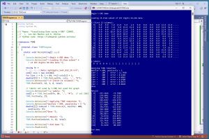 [Click on image for larger view.] Figure 1: The t-SNE Data Reduction Program in Action
The t-SNE algorithm is applied to the source data, resulting in 15 items with just two columns. The reduced data is plotted as an XY graph where the first column is used as x values and the second column is used as the y values. The graph shows three distinct groups of data items as expected.
This article assumes you have intermediate or better programming skill but doesn't assume you know anything about t-SNE data visualization. The demo is implemented using C#, but you should be able to refactor the demo code to another C-family language if you wish.
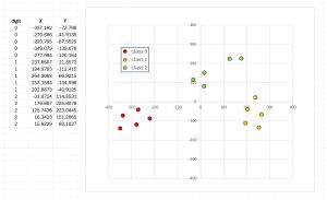 [Click on image for larger view.] Figure 2: The Reduced Data Plotted as an XY Graph
The source code for the demo program is too long to be presented in its entirety in this article. The complete code is available in the accompanying file download, and is also available online. All normal error checking has been removed to keep the main ideas as clear as possible.
The UCI Digits Dataset
The UCI Digits dataset contains crude 8-by-8 images of handwritten digits '0' through '9'. Each image is stored as a comma-delimited row of 64 pixels with integer grayscale values between 0 (white) and 16 (black), followed by the class label (digit represented) from 0 to 9. The UCI Digits dataset is sometimes called the optdigits ("optical digits") dataset.
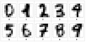 [Click on image for larger view.] Figure 3: Example UCI Digits Dataset Images
The full dataset has 3,823 training images and 1,797 test images. The images in Figure 3 show 10 representative data items. The 15-item dataset used in the demo is the first five '0' images from the test dataset, followed by the first '1' images, followed by the first five '2' images.
The 15-item dataset is presented in Listing 1. To be displayed more easily on a web page, the data has a backslash and newline inserted every eight pixel values. To run the demo, you must delete the backslash-newline characters so that the 64 pixel values and the class label are on one line per image.
Listing 1: The Demo Dataset
# optdigits_test_012_15.txt
# UCI digits, just 5 each of '0', '1', '2'
# 64 pixel values in [0,16] then digit [0,1,2]
#
# remove the \-newline characters so that
# each line has 64 pixel values followed by
# the class label (0, 1, 2)
#
0,0,5,13,9,1,0,0,\
0,0,13,15,10,15,5,0,\
0,3,15,2,0,11,8,0,\
0,4,12,0,0,8,8,0,\
0,5,8,0,0,9,8,0,\
0,4,11,0,1,12,7,0,\
0,2,14,5,10,12,0,0,\
0,0,6,13,10,0,0,0, 0
#
0,0,1,9,15,11,0,0,\
0,0,11,16,8,14,6,0,\
0,2,16,10,0,9,9,0,\
0,1,16,4,0,8,8,0,\
0,4,16,4,0,8,8,0,\
0,1,16,5,1,11,3,0,\
0,0,12,12,10,10,0,0,\
0,0,1,10,13,3,0,0, 0
#
0,0,3,13,11,7,0,0,\
0,0,11,16,16,16,2,0,\
0,4,16,9,1,14,2,0,\
0,4,16,0,0,16,2,0,\
0,0,16,1,0,12,8,0,\
0,0,15,9,0,13,6,0,\
0,0,9,14,9,14,1,0,\
0,0,2,12,13,4,0,0, 0
#
0,0,10,14,11,3,0,0,\
0,4,16,13,6,14,1,0,\
0,4,16,2,0,11,7,0,\
0,8,16,0,0,10,5,0,\
0,8,16,0,0,14,4,0,\
0,8,16,0,1,16,1,0,\
0,4,16,1,11,15,0,0,\
0,0,11,16,12,3,0,0, 0
#
0,0,6,14,10,2,0,0,\
0,0,15,15,13,15,3,0,\
0,2,16,10,0,13,9,0,\
0,1,16,5,0,12,5,0,\
0,0,16,3,0,13,6,0,\
0,1,15,5,6,13,1,0,\
0,0,16,11,14,10,0,0,\
0,0,7,16,11,1,0,0, 0
#
#
0,0,0,12,13,5,0,0,\
0,0,0,11,16,9,0,0,\
0,0,3,15,16,6,0,0,\
0,7,15,16,16,2,0,0,\
0,0,1,16,16,3,0,0,\
0,0,1,16,16,6,0,0,\
0,0,1,16,16,6,0,0,\
0,0,0,11,16,10,0,0, 1
#
0,0,0,0,14,13,1,0,\
0,0,0,5,16,16,2,0,\
0,0,0,14,16,12,0,0,\
0,1,10,16,16,12,0,0,\
0,3,12,14,16,9,0,0,\
0,0,0,5,16,15,0,0,\
0,0,0,4,16,14,0,0,\
0,0,0,1,13,16,1,0, 1
#
0,0,0,2,16,16,2,0,\
0,0,0,4,16,16,2,0,\
0,1,4,12,16,12,0,0,\
0,7,16,16,16,12,0,0,\
0,0,3,10,16,14,0,0,\
0,0,0,8,16,12,0,0,\
0,0,0,6,16,16,2,0,\
0,0,0,2,12,15,4,0, 1
#
0,0,0,0,12,5,0,0,\
0,0,0,2,16,12,0,0,\
0,0,1,12,16,11,0,0,\
0,2,12,16,16,10,0,0,\
0,6,11,5,15,6,0,0,\
0,0,0,1,16,9,0,0,\
0,0,0,2,16,11,0,0,\
0,0,0,3,16,8,0,0, 1
#
0,0,0,1,11,9,0,0,\
0,0,0,7,16,13,0,0,\
0,0,4,14,16,9,0,0,\
0,10,16,11,16,8,0,0,\
0,0,0,3,16,6,0,0,\
0,0,0,3,16,8,0,0,\
0,0,0,5,16,10,0,0,\
0,0,0,2,14,6,0,0, 1
#
#
0,0,0,4,15,12,0,0,\
0,0,3,16,15,14,0,0,\
0,0,8,13,8,16,0,0,\
0,0,1,6,15,11,0,0,\
0,1,8,13,15,1,0,0,\
0,9,16,16,5,0,0,0,\
0,3,13,16,16,11,5,0,\
0,0,0,3,11,16,9,0, 2
#
0,0,5,12,1,0,0,0,\
0,0,15,14,7,0,0,0,\
0,0,13,1,12,0,0,0,\
0,2,10,0,14,0,0,0,\
0,0,2,0,16,1,0,0,\
0,0,0,6,15,0,0,0,\
0,0,9,16,15,9,8,2,\
0,0,3,11,8,13,12,4, 2
#
0,0,8,16,5,0,0,0,\
0,1,13,11,16,0,0,0,\
0,0,10,0,13,3,0,0,\
0,0,3,1,16,1,0,0,\
0,0,0,9,12,0,0,0,\
0,0,3,15,5,0,0,0,\
0,0,14,15,8,8,3,0,\
0,0,7,12,12,12,13,1, 2
#
0,0,0,5,14,12,2,0,\
0,0,7,15,8,14,4,0,\
0,0,6,2,3,13,1,0,\
0,0,0,1,13,4,0,0,\
0,0,1,11,9,0,0,0,\
0,8,16,13,0,0,0,0,\
0,5,14,16,11,2,0,0,\
0,0,0,6,12,13,3,0, 2
#
0,0,0,3,15,10,1,0,\
0,0,0,11,10,16,4,0,\
0,0,0,12,1,15,6,0,\
0,0,0,3,4,15,4,0,\
0,0,0,6,15,6,0,0,\
0,4,15,16,9,0,0,0,\
0,0,13,16,15,9,3,0,\
0,0,0,4,9,14,7,0, 2
I saved the 15-item source data as optdigits_test_012_15.txt in a Data directory located in the project root directory. The wacky data file name is intended to indicate that the file contains 15 items from the UCI Digits test data, where the items are class '0', '1' or '2'.
Unlike many machine learning techniques, t-SNE visualization does not require you to normalize the source data. Source data can be normalized, typically using z-score normalization, or min-max normalization, or divide-by-constant normalization. But t-SNE can work directly with raw data because there are no Euclidean distance, or similar, operations where data columns with large magnitude values will overwhelm columns with small magnitudes.
After applying t-SNE to the 15-item UCI Digits subset, the condensed two-dimensional values can be seen on the left side of the graph in Figure 3. The condensed two-dimensional data looks like:
[ 0]   -337.1624  -72.7990
[ 1]   -270.6862  -41.9135
. . .
[14]     15.6229   80.1027
The UCI Digits dataset has class labels, but t-SNE visualization can be applied to data with or without labels. When examining data that has explicit class labels, t-SNE usually does not include the labels as part of the source. As with the demo, class labels are typically used just to verify t-SNE visualization results.
The Demo Program
To create the t-SNE demo program I used Visual Studio 2022 (Community Free Edition). I created a new C# console application and checked the "Place solution and project in the same directory" option. I specified .NET version 8.0. I named the project TSNE. I checked the "Do not use top-level statements" option to avoid the rather annoying program entry point shortcut syntax.
The demo has no significant .NET dependencies and any relatively recent version of Visual Studio with .NET (Core) or the older .NET Framework will work fine. You can also use the Visual Studio Code program if you like.
After the template code loaded into the editor, I right-clicked on file Program.cs in the Solution Explorer window and renamed the file to the slightly more descriptive TSNEProgram.cs. I allowed Visual Studio to automatically rename class Program.
The C# demo program is a refactoring of the original t-SNE program which is written in Python. The source research paper is "Visualizing Data using t-SNE" (2008), by L. van der Maaten and G. Hinton. The original Python implementation was written by van der Maaten and can be found at https://lvdmaaten.github.io/tsne/. The Python implementation is labeled as free to use, modify or redistribute for non-commercial purposes.
The overall program structure is presented in Listing 2. The TSNEProgram class houses the Main() method, which has all the control logic. The TSNE class is a simple wrapper over the Reduce() function that does all the work.
Listing 2: The t-SNE Demo Program Structure
using System;
using System.IO;

namespace TSNE
{
  internal class TSNEProgram
  {
    static void Main(string[] args)
    {
      // load data from file into memory
      // apply the t-SNE Reduce() function
      // show reduced two-dmensional order
    }
  } // Program

  public class TSNE
  {
    // wrapper class for static Reduce() and helpers

    public static double[][] Reduce(double[][] X,
      int maxIter, int perplexity) { . . }

    // ----- two primary helper functions

    private static double[][] ComputeP(double[][] X,
      int perplexity) { . . }

    private static double[] ComputePH(double[] di,
      double beta, out double h) { . . }

    // ------------------------------------------------------
    //
    // 32 secondary helper functions, and one helper class
    //
    // MatSquaredDistances, MatCreate, MatOnes,
    // MatLoad, MatSave, VecLoad,
    // MatShow, MatShow, MatShow, (3 overloads)
    // VecShow, VecShow, MatCopy, MatAdd, MatTranspose,
    // MatProduct, MatDiff, MatExtractRow,
    // MatExtractColumn, VecMinusMat, VecMult, VecTile,
    // MatMultiply, MatMultLogDivide, MatRowSums,
    // MatColumnSums, MatColumnMeans, MatReplaceRow,
    // MatVecAdd, MatAddScalar, MatInvertElements,
    // MatSum, MatZeroOutDiag
    //
    // Gaussian class: NextGaussian()
    //
    // ------------------------------------------------------

  } // class TSNE
} // ns
The Reduce() function calls two primary helper functions, ComputeP() and ComputePH(). I renamed them from the x2p() and Hbeta() Python implementation names. The bulk of the demo program consists of 31 secondary helper functions and a helper class. Most of these secondary helpers are simple and implement functionality that is built in to Python. For example, in Python, if A and B are two NumPy matrices, you can write C = A + B. But when using raw C# you must implement a program-defined function such as:
private static double[][] MatAdd(double[][] A, double[][] B)
{
  int rows = A.Length;
  int cols = A[0].Length;
  double[][] result = MatCreate(rows, cols); // helper
  for (int i = 0; i < rows; ++i)
    for (int j = 0; j < cols; ++j)
      result[i][j] = A[i][j] + B[i][j];
  return result;
}
The Calling Code
The Main() method begins by loading the 15-item UCI Digits subset into memory:
string fn = "..\\..\\..\\Data\\optdigits_test_012_15.txt";
int[] cols = new int[64];
for (int i = 0; i < 64; ++i) cols[i] = i;
double[][] X = TSNE.MatLoad(fn, cols, ',', "#");
Console.WriteLine("\nX (first 12 columns): ");
TSNE.MatShow(X, 12, 1, 6, true);
The arguments passed to the MatLoad() function mean load 64 comma-delimited columns [0] through [63] inclusive, where lines beginning with "#" are comments to be ignored. The arguments to MatShow() mean show the first 12 columns of data, using 1 decimal, with a field width of 6, and show row indices.
The demo loads the class labels in column [64] and displays them like so:
Console.WriteLine("y labels: ");
int[] y = TSNE.VecLoad(fn, 64, "#");  // col [64]
TSNE.VecShow(y, 3);
As mentioned previously, t-SNE does not need labels, and the demo program uses them only to verify that the reduced data accurately reflects the source data.
The source data is reduced and displayed using these statements:
Console.WriteLine("maxIter = 600, perplexity = 5 ");
double[][] reduced = TSNE.Reduce(X, maxIter: 600,
  perplexity: 5);
Console.WriteLine("Result: ");
TSNE.MatShow(reduced, 4, 12, true);
The t-SNE reduction process is iterative. The maximum number of iterations must be determined by trial and error. The demo monitors error/cost every 100 iterations. Preliminary experiments showed that error stopped significantly decreasing at roughly 600 iterations.
The primary hyperparameter for t-SNE reduction is called perplexity. The perplexity value defines how many nearest data items are used during reduction. Perplexity can be thought of as a parameter to tune the balance between preserving the global and the local structure of the data. The t-SNE process is highly sensitive to the perplexity value, and a good value must be determined by trial and error. Because the demo dataset is so small, a small perplexity value of 5 was used. Typical perplexity values are between 5 and 100.
The MatShow() call is an overload and the parameters means display using 4 decimals, width 12, and show row indices. At this point, I manually copied the reduced data values from the running shell and placed them into an Excel spreadsheet to make the graph shown in Figure 2. In a non-demo scenario with a large dataset, I could have saved the reduced data as a comma-delimited text file using the MatSave() function defined in the demo program. Instead of using a manual approach, I could have used one of many ways to programmatically transfer data to an Excel spreadsheet, or to programmatically generate a graph on a WinForms application.
Initialization
A non-trivial task when implementing t-SNE using raw C# is generating Gaussian distributed random values with mean = 0 and standard deviation = 1. Gaussian values are used to initialize the n-by-2 result matrix. The demo program implements a private-scope Gaussian class that is nested inside the main TSNE class. The code is shown in Listing 3.
Listing 3: The Gaussian Class
class Gaussian
{
  private Random rnd;
  private double mean;
  private double sd;

  public Gaussian(double mean, double sd, int seed)
  {
    this.rnd = new Random(seed);
    this.mean = mean;
    this.sd = sd;
  }

  public double NextGaussian()
  {
    double u1 = this.rnd.NextDouble();
    double u2 = this.rnd.NextDouble();
    double left = Math.Cos(2.0 * Math.PI * u1);
    double right = Math.Sqrt(-2.0 * Math.Log(u2));
    double z = left * right;
    return this.mean + (z * this.sd);
  }
} // Gaussian
The Gaussian constructor accepts a mean and standard deviation. The NextGaussian() method returns a single Gaussian distributed value. The Gaussian class implements a simplified version of the clever Box-Muller algorithm.
Wrapping Up
Using t-SNE is just one of several ways to visualize data that has three or more columns. Such systems are often called dimensionality reduction techniques. Principal component analysis (PCA) is similar in some respects to t-SNE. PCA doesn't require any hyperparameters, but PCA visualization results tend to be very good or quite poor.
Another dimensionality reduction technique to visualize data is to use a neural network autoencoder with a central hidden layer that has two nodes. Neural autoencoders require many hyperparameters (number of hidden layers, hidden and output activation functions, learning rate, batch size, maximum epochs) and so a good visualization is more difficult to achieve. But a neural autoencoder can theoretically produce the best visualization.
Although t-SNE is designed to generate reduced two-dimensional data for use in a graph, the technique can generate higher-dimensional data. But this use of t-SNE is relatively rare because PCA and autoencoders are usually a better approach.
The t-SNE technique is computationally expensive and can be very slow when applied to source data that has many (more than 100) columns. For such source data, a common trick is to apply PCA to reduce the data to roughly 50 columns, and then apply t-SNE to reduce to two columns.