The Data Science Lab
Multi-Class Classification Using LightGBM
Dr. James McCaffrey of Microsoft Research provides a full-code, step-by-step machine learning tutorial on how to use the LightGBM system to perform multi-class classification using Python and the scikit-learn library.
A multi-class classification problem is one where the goal is to predict a discrete variable that has three or more possible values. For example, you might want to predict a person's political leaning (conservative, moderate, liberal) from sex, age, state of residence and annual income. There are many machine learning techniques for multi-class classification. One of the most powerful techniques is to use the LightGBM (lightweight gradient boosting machine) system.
LightGBM is a sophisticated, open-source, tree-based system that was introduced in 2017. LightGBM can perform multi-class classification, binary classification (predict one of two possible values), regression (predict a single numeric value) and ranking.
The best way to see where this article is headed is to take a look at the screenshot of a demo program in Figure 1. LightGBM has three programming language interfaces -- C, Python and R. The demo program uses the Python language API. The demo begins by loading the data to analyze into memory. The data looks like:
[1.  24.  0.  29500.]  | 2
[0.  39.  2.  51200.]  | 1
[1.  63.  1.  75800.]  | 0
. . .
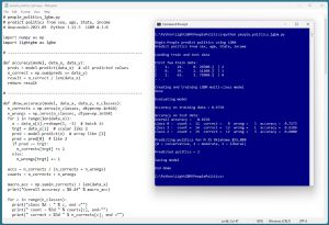 [Click on image for larger view.] Figure 1: LightGBM Multi-Class Classification in Action.
There are 200 items in the training dataset and 40 items in a test dataset. Each line represents a person. The predictor variables are sex, age, state and income. The target class label to predict is political leaning (0 = conservative, 1 = moderate, 2 = liberal).
The demo creates and trains a LightGBM classifier object. The trained model predicts the training data with 97.5 percent accuracy (195 out of 200 correct) and the test data with 82.5 percent accuracy (33 out of 40 correct).
The demo concludes by predicting political leaning for a new, previously unseen person who is male, age 35, from Oklahoma, who make $55,000 a year. The prediction is 2 = liberal.
This article assumes you have intermediate or better programming skill with a C-family language and a basic knowledge of decision tree terminology but does not assume you know anything about LightGBM. The entire source code for the demo program is presented in this article and is also available in the accompanying file download. You can also find the source code and data here.
The Data
The demo program uses a 240-item set of synthetic data. The raw data looks like:
F  24  michigan  29500.00  liberal
M  39  oklahoma  51200.00  moderate
F  63  nebraska  75800.00  conservative
M  36  michigan  44500.00  moderate
F  27  nebraska  28600.00  liberal
. . .
The fields are sex (M, F), age, state (Michigan, Nebraska, Oklahoma), income and political leaning (conservative, moderate, liberal). When using LightGBM, it's best to encode categorical predictors and labels using zero-based ordinal encoding. Unlike most other multi-class classification systems, when using LightGBM, numeric predictor variables can be used as-is. You can normalize numeric predictors using min-max, z-score, or divide-by-constant normalization, but normalization does not help LightGBM models.
You can encode your data in a preprocessing step, or you can encode programmatically while the data is being loaded into memory. The demo uses preprocessing. The comma-delimited encoded data looks like:
1, 24, 0, 29500.00, 2
0, 39, 2, 51200.00, 1
1, 63, 1, 75800.00, 0
0, 36, 0, 44500.00, 1
1, 27, 1, 28600.00, 2
. . .
The 240-item encoded data was split into a 200-item set of training data to create a prediction model and a 40-item set of test data to evaluate the model.
Installing Python and LightGBM
To use the Python language API for LightGBM, you must have Python installed on your machine. I strongly recommend using the Anaconda distribution of Python. The Anaconda distribution contains a Python interpreter and roughly 500 Python packages that are compatible with one another. The demo uses version Anaconda3-2023.09-0, which contains Python version 3.11.5. To install Anaconda on a Windows platform, go here and find installer file Anaconda3-2023.09-0-Windows-x86_64.exe (or newer). Note: it is all-too-easy to download a version that's not compatible with your machine.
Click on the .exe file link to download it to your machine. After the file is on your machine, double-click on the file to start the GUI-based installation process. In most scenarios, you can accept all the default installation values except the one which does not add Anaconda3 to your machine's PATH environment variable -- I recommend adding it so that you don't have to manually edit your system environment variables, or enter long paths on the command line.
You can also follow detailed step-by-step instructions for installing Anaconda Python.
You can verify your Anaconda Python installation by opening a command shell and typing the command "python" (without quotes). You should see a reply message that indicates the version of Python, followed by the Python triple greater-than prompt. You can type "exit()" to quit the interpreter.
If you ever need to uninstall Anaconda on a Windows machine, you can do so by going to the Add or Remove Programs setting and clicking on the Uninstall option.
At the time this article was written, the Anaconda distribution does not contain the LightGBM system, and so it must be installed separately. I strongly recommend using the pip installer program (which is included with Anaconda). To install the most recent version of LightGBM over the internet, open a command shell and type the command "pip install lightgbm." After a few seconds, you should see a message indicating success. To verify, open a command shell and type "python." At the Python prompt, type the command "import lightgbm as L" followed by the command "L.__version__" using double underscores. You should see the version of LightGBM that is installed.
Instead of installing LightGBM over the internet, you can first download the LigbtGBM package to your machine and then install. Go here and search for "lightgbm." The search results will give you a link to a LightGBM package page. Click on the Download Files link. You will go to a page that has a .whl file named like lightgbm-4.3.0-py3-none-win_amd64.whl that you can click on to download the file to your machine. After the download completes, open a command shell, navigate to the directory containing the .whl file and install LightGBM by typing the command "pip install [the .whl file name]."
If you ever need to uninstall LightGBM, you can do so by typing the command "pip uninstall lightgbm." I often use the local-install technique so that I can have a copy of LightGBM on my machine.
The LightGBM Demo Program
The complete demo program is presented in Listing 1. The demo begins by loading the training data into memory:
import numpy as np
import lightgbm as lgbm

def main():
  # 0. get started
  np.random.seed(1)

  # 1. load data
  train_file = ".\\Data\\people_train.txt"
  train_x = np.loadtxt(train_file, usecols=[0,1,2,3],
    delimiter=",", comments="#", dtype=np.float64)
  train_y = np.loadtxt(train_file, usecols=4,
    delimiter=",", comments="#", dtype=np.int64)
. . .
The demo does not use the NumPy random number generator directly, but it's good practice to set the generator seed value anyway in case the program is modified to use the RNG.
The demo assumes that the training and test data files are located in a subdirectory named Data. The comma-delimited data is loaded into NumPy arrays using the loadtxt() function. The predictor values in columns 0, 1, 2, 3 are loaded as type float64 and the labels are loaded as type int64. Lines that begin with "#" are comments and are not loaded.
Listing 1: LightGBM Multi-Class Demo Program
# people_politics_lgbm.py
# predict politics from sex, age, State, income
# Anaconda3-2023.09-0  Python 3.11.5  LightGBM 4.3.0

import numpy as np
import lightgbm as lgbm

# -----------------------------------------------------------

def accuracy(model, data_x, data_y):
  # simple
  preds = model.predict(data_x)  # all predicted values
  n_correct = np.sum(preds == data_y)
  result = n_correct / len(data_x)
  return result

# -----------------------------------------------------------

def show_accuracy(model, data_x, data_y, n_classes):
  # more details
  n_corrects = np.zeros(n_classes, dtype=np.int64)
  n_wrongs = np.zeros(n_classes, dtype=np.int64)
  for i in range(len(data_x)):
    x = data_x[i].reshape(1, -1)  # batch it
    trgt = data_y[i]  # scalar like 2
    pred = model.predict(x)  # array like [2]
    pred = pred[0]  # like 2
    if pred == trgt:
      n_corrects[trgt] += 1
    else:
      n_wrongs[trgt] += 1

  accs = n_corrects / (n_corrects + n_wrongs)
  counts = n_corrects + n_wrongs

  macro_acc = np.sum(n_corrects) / len(data_x)
  print("Overall accuracy = %8.4f" % macro_acc)

  for c in range(n_classes):
    print("class %d : " % c, end ="")
    print(" ct = %3d " % counts[c], end="")
    print(" correct = %3d " % n_corrects[c], end ="")
    print(" wrong = %3d " % n_wrongs[c], end ="")
    print(" acc = %7.4f " % accs[c])

# -----------------------------------------------------------

def confusion_matrix_multi(model, data_x, data_y, n_classes):
  # assumes n_classes is 3 or greater ")
  cm = np.zeros((n_classes,n_classes), dtype=np.int64)
  for i in range(len(data_x)):
    x = data_x[i].reshape(1, -1)  # batch it
    trgt_y = data_y[i]  # scalar like 2
    pred_y = model.predict(x)  # array like [2]
    pred_y = pred_y[0]  # like 2
    cm[trgt_y][pred_y] += 1
  return cm

# -----------------------------------------------------------

def show_confusion(cm):
  # cm created using confusion_matrix_multi()
  dim = len(cm)
  mx = np.max(cm)             # largest count in cm
  wid = len(str(mx)) + 1      # width to print
  fmt = "%" + str(wid) + "d"  # like "%3d"
  for i in range(dim):
    print("actual   ", end="")
    print("%3d:" % i, end="")
    for j in range(dim):
      print(fmt % cm[i][j], end="")
    print("")
  print("------------")
  print("predicted    ", end="")
  for j in range(dim):
    print(fmt % j, end="")
  print("")

# -----------------------------------------------------------

def main():
  # 0. get started
  print("\nBegin People predict politics using LightGBM ")
  print("Predict politics from sex, age, State, income ")
  np.random.seed(1)

  # 1. load data that looks like:
  # sex, age, State, income, politics
  # 1, 24, 0, 29500.00, 2
  # 0, 39, 2, 51200.00, 1
  # . . .
  print("\nLoading train and test data ")
  train_file = ".\\Data\\people_train.txt"
  train_x = np.loadtxt(train_file, usecols=[0,1,2,3],
    delimiter=",", comments="#", dtype=np.float64)
  train_y = np.loadtxt(train_file, usecols=4,
    delimiter=",", comments="#", dtype=np.int64)

  test_file = ".\\Data\\people_test.txt"
  test_x = np.loadtxt(test_file, usecols=[0,1,2,3],
    delimiter=",", comments="#", dtype=np.float64)
  test_y = np.loadtxt(test_file, usecols=4,
    delimiter=",", comments="#", dtype=np.int64)

  np.set_printoptions(precision=0, suppress=True,
    floatmode='fixed')
  print("\nFirst few train data: ")
  for i in range(3):
    print(train_x[i], end="")
    print("  | " + str(train_y[i]))
  print(". . . ")

  # 2. create and train model
  print("\nCreating and training LGBM multi-class model ")
  params = {
    # 'objective': 'multiclass',  # not needed
    'boosting_type': 'gbdt',  # default
    'num_leaves': 31,  # default
    'max_depth':-1,  # default (unlimited)
    'n_estimators': 50,  # default = 100
    'learning_rate': 0.05,  # default = 0.10
    'min_data_in_leaf': 5,  # default = 20
    'random_state': 0,
    'verbosity': -1  # only fatal. default = 1 error, warn
  }
  model = lgbm.LGBMClassifier(**params)  # scikit API
  model.fit(train_x, train_y)
  print("Done ")

  # 3. evaluate model
  print("\nEvaluating model ")

  # 3a. using a coarse function
  train_acc = accuracy(model, train_x, train_y)
  print("\nAccuracy on training data = %0.4f " % train_acc)
  test_acc = accuracy(model, test_x, test_y)
  print("Accuracy on test data = %0.4f " % test_acc)

  # 3b. using a detailed function
  print("\nAccuracy on test data: ")
  show_accuracy(model, test_x, test_y, n_classes=3)

  # 3c. using a confusion matrix
  print("\nConfusion matrix for test data: ")
  cm = confusion_matrix_multi(model, test_x,
    test_y, n_classes=3)
  show_confusion(cm)

  # 4. use model
  print("\nPredicting politics for M 35 Oklahoma $55,000 ")
  print("(0 = conservative, 1 = moderate, 2 = liberal) ")
  x = np.array([[0, 35, 2, 55000.00]], dtype=np.float64)
  pred = model.predict(x)
  print("\nPredicted politics = " + str(pred[0]))

  # 5. save model
  import pickle
  print("\nSaving model ")
  pth = ".\\Models\\politics_model.pkl"
  with open(pth, "wb") as f:
    pickle.dump(model, f)

  # with open(pth, "rb") as f:
  #   model2 = pickle.load(f)
  #
  # x = np.array([[0, 35, 2, 55000.00]], dtype=np.float64)
  # pred = model2.predict(x)
  # print("\nPredicted politics = " + str(pred[0]))

  print("\nEnd demo ")

if __name__ == "__main__":
  main()
The test data is loaded into memory as arrays test_x and test_y in the same way as the training data. Next, the demo displays the first three lines of the training data as a sanity check:
  np.set_printoptions(precision=0, suppress=True,
    floatmode='fixed')
  print("First few train data: ")
  for i in range(3):
    print(train_x[i], end="")
    print("  | " + str(train_y[i]))
  print(". . . ")
In a non-demo scenario, you might want to display all the data.
Creating and Training the LightGBM Model
The demo program creates and trains a LightGBM multi-class classifier using these statements:
  # 2. create and train model
  print("Creating and training LGBM multi-class model ")
  params = {
    # 'objective': 'multiclass',  # not needed
    'boosting_type': 'gbdt',  # default
    'num_leaves': 31,  # default
    'max_depth': -1,  # default (unlimited)
    'n_estimators': 50,  # default = 100
    'learning_rate': 0.05,  # default = 0.10
    'min_data_in_leaf': 5,  # default = 20
    'random_state': 0,
    'verbosity': -1  # only fatal. default = 1 error, warn
  }
  model = lgbm.LGBMClassifier(**params)
  model.fit(train_x, train_y)
The classifier object is named model and is instantiated by setting up its parameters as a Python Dictionary collection named params. The main challenge when using LightGBM is wading through the dozens of parameters. The LGBMClassifier class/object has 19 parameters (num_leaves, max_depth and so on) and behind the scenes there are 57 Learning Control Parameters (min_data_in_leaf, bagging_fraction and so on), for a total of 76 parameters to deal with.
Documentation for the parameters can be found here and here.
Because the number of parameters is not manageable, you must rely on the default values and then try to find the handful of parameters that will create a good model. Based on my experience, the three most important parameters to explore and modify are n_estimators, min_data_in_leaf and learning_rate.
A LightGBM classifier is made up of n_estimators (default value is 100), relatively small decision trees that are called weak learners, or sometimes base learners. The weak trees are constructed sequentially where each tree uses gradients of the error from the previous tree. If the value of n_estimators is too small, then there aren't enough weak learners to create a model that predicts well (underfit). If the value of n_estimators is too large, then the model will overfit the training data and predict poorly on new, previously unseen data items.
The num_leaves parameter controls the overall size of the weak learner trees. The default value of 31 translates to a balanced tree that has five levels with 1, 2, 4, 8, 16 leaf nodes respectively. An unbalanced tree might have more levels. Weak learners that are too small might underfit, too large might overfit.
The max_depth parameter controls the number of levels that each weak learner has. The default value is -1, which means that there is no explicit limit. In most cases, the num_leaves parameter will prevent the depth of the weak learners from becoming too large.
The min_data_in_leaf parameter controls the size of the leaf nodes in the weak learners. The default value of 20 means that each leaf node must have at least 20 associated data items. For a relatively small set of training data, the default greatly reduces the number of leaf nodes. For the demo with 200 training items, there would be a maximum of 200 / 20 = 10 leaf nodes, which would likely underfit the model and lead to poor prediction accuracy. The demo modifies the value of min_data_in_leaf from 20 to 5, which gave much better results.
To recap, the n_estimators parameter controls the overall number of weak tree learners. The key parameters to control the size and shape of the weak learners are num_leaves, max_depth and min_data_in_leaf. Based on my experience, I typically experiment with n_estimators (the default value of 100 is often too large for small datasets) and min_data_in_leaf (the default of 20 is often too large for small datasets). I usually leave the num_leaves and max_depth parameter values at their default values of 31 and -1 (unlimited) respectively unless the model just doesn't predict well.
The demo modifies the learning_rate parameter from the default value of 0.10 to 0.05. The learning rate controls how much each weak learner tree changes from the previous learner. The effect of changing the learning_rate can vary quite a bit depending on the size and shape of the weak learners, but as a rule of thumb, smaller values work better for smaller datasets.
The demo modifies the value of the random_state parameter from its default value of None (Python's version of null) to 0. The None value means that results are not reproducible due to the random initialization component of the training process. Any value other than None will give (mostly) reproducible results, subject to multi-threading issues.
The demo modifies the value of the verbosity parameter from its default value of 1 to -1. The default value of 1 prints warning messages, regular error messages and fatal error messages. The demo value of -1 prints only fatal error messages. I did this only to keep the output small so I could take a screenshot. In a non-demo scenario you should leave the verbosity value at 1 in most situations.
After setting up the parameter values in a Dictionary collection, they are passed to the LGBMClassifier using the Python ** syntax, which means unpack the values to parameters. Parameter values can be passed directly, for example model = lgbm.LGBMClassifier(n_estimators = 50, learning_rate = 0.05 and so on), but because there are so many parameters, this approach is rarely used.
The model is trained using the fit() method. Almost too easy because all the work is done when setting up the parameters.
Evaluating the Model
It's possible to evaluate a trained LightGBM multi-class model in several ways. The most basic approach is to compute prediction accuracy (number correct predictions divided by total number of predictions) on the training and test data. The demo program defines an accuracy() function where the key statements are:
preds = model.predict(data_x)  # all predicted values
n_correct = np.sum(preds == data_y)
result = n_correct / len(data_x)
The output of the simple accuracy() function is:
Accuracy on training data = 0.9750
Accuracy on test data = 0.8250
This set-based approach is fast, but iterating through each data item instead allows you to see exactly which items are incorrectly predicted.
The demo defines a show_accuracy() function that gives more detailed information. The output of the show_accuracy() function is:
Accuracy on test data:
Overall accuracy =   0.8250
class 0 :  ct =  11  correct =   8  wrong =   3  acc =  0.7273
class 1 :  ct =  14  correct =  13  wrong =   1  acc =  0.9286
class 2 :  ct =  15  correct =  12  wrong =   3  acc =  0.8000
For multi-class classification problems, it's more or less standard practice to compute and display a confusion matrix that shows where incorrect predictions have been made. The demo defines a confusion_matrix_multi() function that computes a confusion matrix and a show_confusion() function that displays the matrix. The demo output is:
Confusion matrix for test data:
actual     0:  8  2  1
actual     1:  1 13  0
actual     2:  2  1 12
------------
predicted      0  1  2
The entries off the main diagonal are incorrect predictions. For example, the 2 value at row [0] and column [1] indicates that there were 2 data items that have true political leaning = 0 (conservative) but were predicted to be class 1 (moderate).
The LightGBM Python API is integrated with the scikit-learn machine learning package. The scikit-learn package is included in the Anaconda distribution and so you can directly call built-in scikit-learn modules. For example, you can get a confusion matrix using these statements:
from sklearn.metrics import confusion_matrix
pred_y = model.predict(test_x)  # all predicteds
cm = confusion_matrix(test_y, pred_y)
print(cm)
Or you can get detailed evaluation (a bit too detailed in my opinion) like so:
from sklearn.metrics import classification_report
pred_y = model.predict(test_x)  # all predicteds
report = classification_report(test_y, pred_y,
  labels=[0, 1, 2])
print(report)
The ability to use built-in scikit-learn library modules is powerful but has a bit of a learning curve if you're not familiar with the library.
Using and Saving the LightGBM Model
Using a trained LightGBM classifier is simple, subject to two minor syntax details. Example calling code is:
x = np.array([[0, 35, 2, 55000.00]], dtype=np.float64)  # 2D
pred = model.predict(x)
print("Predicted politics = " + str(pred[0]))
Notice that the input x values have double square brackets to make the input a 2D matrix, which the predict() method requires. Alternatively, you can declare a 1D vector and then reshape it to 2D:
x = np.array([0, 35, 2, 55000.00], dtype=np.float64)  # 1D
x = x.reshape(1, -1)  # 1 row, n cols 2D
pred = model.predict(x)
The return value from the predict() method is an array rather than a scalar value. So, when the input is a single data item, and you want just the single predicted class, you can access the class at index [0] like so:
pred = model.predict(x)
print("Predicted politics = " + str(pred[0]))
Alternatively:
pred = model.predict(x)  # array
pred = pred[0]           # scalar
print("Predicted politics = " + str(pred))
The demo program saves the trained LightGBM in binary format using the Python pickle library. (In ordinary English, the word "pickle" means to preserve). The calling code is:
import pickle
print("Saving model ")
pth = ".\\Models\\politics_model.pkl"
with open(pth, "wb") as f:
  pickle.dump(model, f)
The code assumes the existence of a subdirectory named Models. The "wb" argument means "write to file as binary." The "pkl" extension is common, but any extension name can be used.
A LightGBM model saved using pickle can be loaded into memory from another program and used like so:
pth = ".\\Models\\politics_model.pkl"
with open(pth, "rb") as f:
  model2 = pickle.load(f)
x = np.array([[0, 35, 2, 55000.00]], dtype=np.float64)
pred = model2.predict(x)
There are other ways to save a trained LightGBM model, but the pickle approach is the easiest and the most common.
Wrapping Up
The LightGBM system was inspired by the XGBoost (extreme gradient boosting) system, which in turn was inspired by earlier tree boosting algorithms. The "boosting" term of the LightGBM name refers to the technique of combining several weak learners into one strong learning model. The "gradient" term refers to the technique of using the Calculus gradient of the error of a weak learner to construct the next weak learner in the model sequence. The "machine" term is an old way to indicate that a system is a machine learning one rather than a classical statistics one.
Arguably, the two most powerful techniques for multi-class classification on non-trivial datasets are neural networks and tree boosting. In some recent multi-class classification challenges, LightGBM entries have dominated the contest leader board. This may be due, in part, to the fact that LightGBM can be used out-of-the-box, which leaves a lot of time for hyperparameter fine-tuning. Using a neural network classifier requires significantly more background knowledge and effort.