Neural Network Lab
Neural Network Training Using Back-Propagation
James McCaffrey explains the common neural network training technique known as the back-propagation algorithm.
Neural networks can be used to classify data and make predictions. For example, you might want to predict the political party affiliation (Democrat, Republican, Independent) of a person based on factors such as their age, annual income, sex and so on. Behind the scenes, a neural network can be thought of as a complicated mathematical function that has various constants called weights and biases, which must be determined. The process of finding the set of weights and bias values that best match your existing data is called training the neural network. There are many ways to train a neural network. By far the most common neural network training technique (but not necessarily the best) is to use what's called the back-propagation algorithm.
Although there are many good references available that explain the interesting mathematics of back-propagation training, there are very few resources that describe the practical issues involved in implementing back-propagation training. In this article, I describe exactly how to train a neural network using back-propagation. This article assumes you have a basic familiarity with neural networks and back-propagation, and at least intermediate-level programming skills.
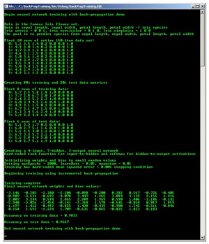
The best way to see where this article is headed is to take a look at Figure 1. The demo program analyzes a set of data about three different species of Iris flowers. The possible species are Iris setosa, Iris versicolor and Iris virginica. The goal is to predict the species from four numeric values: sepal (the green covering) length and width, and petal length and width. This flower data may not excite you, but it's a famous data set that has been used as an example for many decades.
 [Click on image for larger view.]
Figure 1. Neural network training using back-propagation.
[Click on image for larger view.]
Figure 1. Neural network training using back-propagation.
The demo program starts by splitting the data set, which consists of 150 items, into a training set of 120 items (80 percent) and a test set of 30 items (20 percent). Next, the demo creates a neural network with four input nodes (one for each numeric input), seven hidden nodes and three output nodes (one for each possible output class). The neural network uses the hyperbolic tangent function for hidden node activation, and the softmax function for output node activation.
The neural network's weights and bias values are initialized to small (between 0.001 and 0.0001) random values. Then the back-propagation algorithm is used to search for weights and bias values that generate neural network outputs that most closely match the output values in the training data. Training with back-propagation is an iterative process. In the demo, the training process stops after 2,000 iterations, or when a mean squared error term drops below 0.001. The behavior of the back-propagation algorithm depends in part on the values of a learning rate (set to 0.05 in the demo) and a momentum (set to 0.01).
After the training process is completed, the demo displays the values of the neural network's 59 weights and biases that were determined by the training process. The demo finishes by computing the neural network's prediction accuracy on the training data set, which is 0.9833 (118 correct out of 120), and the prediction accuracy on the test data (29 out of 30 = 0.9667).
Coding a neural network from scratch is a lot of work. Why not just use an existing tool with a nice GUI? In many cases using an existing tool is your best option, but an existing tool can be difficult to integrate into a software system, it might be impossible to customize and it might have hidden copyright issues. Additionally, coding a neural network from scratch can give you a better understanding of exactly how existing tools work. And you may just find neural networks interesting in their own right.
The demo program is too long to present here in its entirety, but the entire source code is available in the download accompanying this article. I coded the demo using C#, but you should be able to refactor my code to another language without too much difficulty. I've removed most normal error checking to keep the size of the code smaller and the main ideas clear.
The Data
The Iris data set consists of 150 data items. The raw data, which is available from many sources on the Internet, resembles:
5.1, 3.5, 1.4, 0.2, Iris setosa
7.0, 3.2, 4.7, 1.4, Iris versicolor
6.3, 3.3, 6.0, 2.5, Iris virginica
4.9, 3.0, 1.4, 0.2, Iris setosa
...
There are 50 data points for each species. Because neural networks work with numeric data, the categorical species information must be converted to numeric data. When performing neural network classification, the classes to be predicted should be encoded using 1-of-N encoding. With three classes, one possibility is class 0 = (0, 0, 1), class 1 = (0, 1, 0) and class 2 = (1, 0, 0). To simplify the system, the data set is stored directly in 1-of-N encoded format:
5.1, 3.5, 1.4, 0.2, 0, 0, 1
7.0, 3.2, 4.7, 1.4, 0, 1, 0
6.3, 3.3, 6.0, 2.5, 1, 0, 0
4.9, 3.0, 1.4, 0.2, 0, 0, 1
...
In short, the demo program assumes a very particular data format: no header line, comma-delimited, 1-of-N encoded dependent-variable data located in the last three columns, and so on. Most existing neural network tools allow you to specify exactly how your data is formatted. In general, when working with neural networks, dealing with the format of data is not conceptually difficult, but it can be quite tedious and time-consuming.
Program Structure
The overall structure of the demo program, with some WriteLine statements removed and minor edits to save space, is presented in Listing 1. To create the demo, I launched Visual Studio and created a new console application project named BackPropTraining. After the template code loaded, I renamed file Program.cs to BackPropTrainingProgram.cs and Visual Studio automatically renamed class Program. At the top of the source code, I deleted all references to namespaces except the reference to the System namespace.
Listing 1. Overall program structure.
using System;
namespace BackPropTraining
{
  class BackPropTrainingProgram
  {
    static void Main(string[] args)
    {
      Console.WriteLine("Begin back-propagation demo\n");
      double[][] allData = new double[150][];
      allData[0] = new double[] { 5.1, 3.5, 1.4, 0.2, 0, 0, 1 };
      allData[1] = new double[] { 4.9, 3.0, 1.4, 0.2, 0, 0, 1 };
      ...
      allData[149] = new double[] { 5.9, 3.0, 5.1, 1.8, 1, 0, 0 };

      Console.WriteLine("First 10 rows of entire 150-item data set:");
      ShowMatrix(allData, 10, 1, true);

      Console.WriteLine("Creating 80% train, 20% test data matrices");
      double[][] trainData = null;
      double[][] testData = null;
      MakeTrainTest(allData, out trainData, out testData);

      Console.WriteLine("First 8 rows of training data:");
      ShowMatrix(trainData, 8, 1, true);
      Console.WriteLine("First 6 rows of test data:");
      ShowMatrix(testData, 6, 1, true);

      Console.WriteLine("Creating a 4-7-3 neural network");
      Console.WriteLine("Hard-coded tanh and softmax");
      const int numInput = 4;
      const int numHidden = 7;
      const int numOutput = 3;
      NeuralNetwork nn = new NeuralNetwork(numInput, numHidden, numOutput);

      Console.WriteLine("Initializing weights and bias to random values");
      nn.InitializeWeights();

      int maxEpochs = 2000;
      double learnRate = 0.05;
      double momentum = 0.01;
      Console.WriteLine("Setting maxEpochs = 2000, learnRate = 0.05, " +
       " momentum = 0.01");
      Console.WriteLine("Hard-coded MSE < 0.001 stopping");

      Console.WriteLine("Beginning training using back-propagation\n");
      nn.Train(trainData, maxEpochs, learnRate, momentum);
      Console.WriteLine("Training complete");

      double[] weights = nn.GetWeights();
      Console.WriteLine("Final neural network weights and bias values:");
      ShowVector(weights, 10, 3, true);

      double trainAcc = nn.Accuracy(trainData);
      Console.WriteLine("Accuracy on training data = " + trainAcc);

      double testAcc = nn.Accuracy(testData);
      Console.WriteLine("Accuracy on test data = " + testAcc);

      Console.WriteLine("End back-propagation demo\n");
      Console.ReadLine();
    } // Main

    static void MakeTrainTest(double[][] allData, out double[][] trainData,
      out double[][] testData) { . . }
    static void ShowVector(double[] vector, int valsPerRow, int decimals,
      bool newLine) { . . }
    static void ShowMatrix(double[][] matrix, int numRows, int decimals,
      bool newLine) { . . }
  } // class Program

  public class NeuralNetwork { . . }
} // ns
After some preliminary WriteLine messages, the demo sets up the pre-encoded Iris source data in an array-of-arrays style matrix:
double[][] allData = new double[150][];
allData[0] = new double[] { 5.1, 3.5, 1.4, 0.2, 0, 0, 1 };
allData[1] = new double[] { 4.9, 3.0, 1.4, 0.2, 0, 0, 1 };
...
allData[149] = new double[] { 5.9, 3.0, 5.1, 1.8, 1, 0, 0 };
In most cases, neural network data will be stored in a text file or a SQL table. In such situations you can either load all data into memory, or stream through the external data.
The demo program uses what's called hold-out validation, in which the source data is divided into a training set (used to determine the neural network weights and bias values) and a test set (used after training to get an estimate of how accurate the neural network prediction model will be on new, previously unseen data). The demo calls a utility method MakeTrainTest, which randomly assigns 80 percent of the data to a training matrix and 20 percent of the data to a test matrix:
double[][] trainData = null;
double[][] testData = null;
MakeTrainTest(allData, out trainData, out testData);
The demo instantiates a 3-7-4 neural network where the number of hidden nodes, 7, is arbitrary:
const int numInput = 4;
const int numHidden = 7;
const int numOutput = 3;
NeuralNetwork nn = new NeuralNetwork(numInput, numHidden, numOutput);
Determining the optimal number of hidden nodes is basically an unsolved problem in neural network research, and so trial and error is generally used.
A 4-7-3 neural network will have 4*7 + 7*3 = 49 weights and 7+3 = 10 biases. The demo initializes each weight and bias to a small random value using method InitializeWeights:
nn.InitializeWeights();
This call could've been placed inside the neural network's constructor. The statements that perform training using back-propagation are:
int maxEpochs = 2000;
double learnRate = 0.05;
double momentum = 0.01;
nn.Train(trainData, maxEpochs, learnRate, momentum);
Variable maxEpochs sets a limit on the number of times the back-propagation algorithm iterates through the training data set. Variable learnRate controls how fast the weights and bias values change. Variable momentum adds an additional boost to the rate of change of the weights and bias values.
After the neural network has been trained, the network's predictive accuracy is computed:
double trainAcc = nn.Accuracy(trainData);
double testAcc = nn.Accuracy(testData);
The neural network's accuracy on the training data isn't entirely relevant because by using a very large number of hidden nodes, and training long enough, any data set can in theory be matched with 100 percent accuracy. The relevant measure of accuracy is the predictive accuracy of the neural network on the test data. This gives an estimate of how well the neural network will perform on new data.
Making the Train-Test Data
Method MakeTrainTest accepts as input the entire 150-item data set (as a matrix) and returns, as out parameters, a 120-item training set and a 30-item test set, both as matrices. In pseudo-code:
generate an array of index values from 0 to 149
shuffle the index values to a random order
loop i = each cell in shuffled array
  get idx = curr cell value (an index into the source data)
  if i < 120
    allocate a row of data in training matrix
    copy row[idx] of source data to training matrix
  else if i >= 120
    allocate a row of data in test matrix
    copy row[idx] of source data to test matrix
  end if
end loop
The implementation generates new matrices for the training data and the test data. It isn't necessary to make a copy of the source data; an alternative is to just maintain an array of shuffled index values into the source data. Then instead of accessing the training and test data directly through distinct matrices, you could access them indirectly through the idx reference in the shuffled index array and into the entire data set. For example:
for (int i = 0; i < 120; ++i) // Each virtual training data item
{
  int idx = shuffled[i];
  // AllData[idx] represents a training data item
  ...
}
For small data sets I prefer the simplicity of duplicating source data into the training and test matrices, but if machine memory is a concern I'll sometimes resort to the indirect-access technique.
The demo program doesn't normalize the numeric input. In most neural network classification scenarios, normalizing the independent x-data yields better results. But in this case, the values of the four independent variables -- sepal length and width, and petal length and width -- are all relatively close, so there's no need to normalize the training and test data.
The Neural Network Class
The structure of the class that defines a neural network designed for back-propagation is presented in Listing 2.
Listing 2. Neural network class.
public class NeuralNetwork
{
  private static Random rnd;

  private int numInput;
  private int numHidden;
  private int numOutput;

  private double[] inputs;
  private double[][] ihWeights;
  private double[] hBiases;
  private double[] hOutputs;
  private double[][] hoWeights;
  private double[] oBiases;
  private double[] outputs;

  private double[] oGrads; // Output gradients for back-prop
  private double[] hGrads; // Hidden gradients for back-prop
  private double[][] ihPrevWeightsDelta;  // For momentum back-prop
  private double[] hPrevBiasesDelta;
  private double[][] hoPrevWeightsDelta;
  private double[] oPrevBiasesDelta;

  public NeuralNetwork(int numInput, int numHidden,
    int numOutput) { . . }
  private static double[][] MakeMatrix(int rows, int cols) { . . }
  public override string ToString() { . . }

  public void SetWeights(double[] weights) { . . }
  public void InitializeWeights() { . . }
  public double[] GetWeights() { . . }

  private double[] ComputeOutputs(double[] xValues)
  private static double HyperTanFunction(double x) { . . }
  private static double[] Softmax(double[] oSums) { . . }

  private void UpdateWeights(double[] tValues, double learnRate,
    double momentum) { . . }

  public void Train(double[][] trainData, int maxEprochs,
    double learnRate, double momentum) { . . }
  private static void Shuffle(int[] sequence) { . . }
  private double MeanSquaredError(double[][] trainData)

  public double Accuracy(double[][] testData) { . . }
  private static int MaxIndex(double[] vector) { . . }
}
Static class member rnd is a random number generator that's used by method InitializeWeights to set initial values for the weights and biases, and by helper method Shuffle so that training data can be processed in random order. In addition to the seven basic neural network arrays that are used to compute outputs for a given set of inputs, weights and bias values, it's necessary to include additional arrays that are used by the back-propagation algorithm. Arrays oGrads and hGrads hold the error gradients for output nodes and hidden nodes, respectively. Arrays ihPrevWeightsDelta, hPrevBiasDelta, hoPrevWeightsDelta and oPrevBiasesDelta are needed by the momentum part of the back-propagation algorithm.
Method ComputeOutputs copies input values into the neural network, and uses the current set of weights and bias values to compute the output values. Method ComputeOutputs calls methods HyperTanFunction and Softmax to perform activation for the hidden-layer and output-layer nodes. Method UpdateWeights uses the back-propagation algorithm to modify the current weights and bias values, using the current input and output values, so that new output values will more closely match a set of target values.
Method Train iteratively calls ComputeOutputs and UpdateWeights for each training data item. Method Train calls method Shuffle so that training data is processed in random order, and calls method MeanSquaredError so that training can stop if some small overall error value is reached.
Method Accuracy uses the current set of weights and bias values to count the percentage of correct predictions. Method Accuracy calls helper method MaxIndex, which determines the cell index in an array that holds the largest value.
Training the Neural Network
The code for method Train begins:
public void Train(double[][] trainData, int maxEpochs,
  double learnRate, double momentum)
{
  int epoch = 0;
  double[] xValues = new double[numInput];
  double[] tValues = new double[numOutput];

  int[] sequence = new int[trainData.Length];
  for (int i = 0; i < sequence.Length; ++i)
    sequence[i] = i;
...
Variable epoch is a loop counter. Arrays xValues and tValues will hold the input values and the correct output (target) values for a particular training data item. Recall that a training data item looks like 5.1, 3.5, 1.4, 0.2, 0, 0, 1, where the first four values are inputs, and the last three values are 1-of-N encoded target values. In neural network literature, target values are sometimes called desired values or ideal values.
Array sequence will be used to generate a random ordering of training items on each pass through the main training loop, which is:
while (epoch < maxEpochs) {
  double mse = MeanSquaredError(trainData);
  if (mse < 0.001) break; // Consider passing in as parameter

  Shuffle(sequence);
  for (int i = 0; i < trainData.Length; ++i) {
    int idx = sequence[i];
    Array.Copy(trainData[idx], xValues, numInput);
    Array.Copy(trainData[idx], numInput, tValues, 0, numOutput);
    ComputeOutputs(xValues);
    UpdateWeights(tValues, learnRate, momentum);
  }
  ++epoch;
}
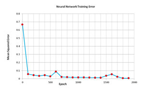
The training loop is controlled by variable maxEpochs. At the top of the loop, method MeanSquaredError scans the entire training set and an overall error value is computed. If this error is less than 0.001, the training loop exits early. Because computing the mean squared error is an expensive operation, an alternative is to compute error only once every 100 or so epochs. The graph in Figure 2 shows how the mean squared error changes over time for the demo program.
 [Click on image for larger view.]
Figure 2. Neural network training error.
[Click on image for larger view.]
Figure 2. Neural network training error.
For each epoch, every data item in the training set is processed. First, helper method Shuffle rearranges the sequence array into a random order. A training item is selected, and inputs and targets are extracted. The inputs are fed to method ComputeOutputs. Then method UpdateWeights uses the target values to modify the weights and bias values so that the outputs more closely match the target values.
This particular training approach, where back-propagation updates occur for every training item based on the difference between the computed outputs and the target outputs, has several different names including sequential training, incremental training and online training. An alternative is to read all training data, accumulate an overall difference between all computed outputs and all target outputs, and then perform a single back-propagation update. This approach is usually called batch training. In my opinion, there's convincing research that suggests incremental training is superior to batch training when using back-propagation.
Measuring Accuracy
After a neural network has been trained, the next step is to estimate how well the model will perform on new data. Method Accuracy computes the percentage of correct predictions that are made on the test data that was withheld from training. Method Accuracy uses a winner-takes-all approach that's best explained by example. Suppose a set of input values is (5.0, 4.0, 1.0, 2.0) and the target correct output is (0, 1, 0), which represents Iris versicolor in 1-of-N encoded form. Now suppose that, after training, the neural network computed output values for inputs (5.0, 4.0, 1.0, 2.0) are (0.15, 0.60, 0.25). Notice that because the demo program uses softmax activation, the output values are all between 0 and 1, and sum to 1.0, and so can be interpreted as probabilities. Therefore, in this case, because the highest probability is 0.60, I'd conclude that outputs (0.15, 0.60, 0.25) map to (0, 1, 0), and the predicted value is correct. But suppose instead that the computed outputs were (0.55, 0.20, 0.25). That output set would map to (1, 0, 0) and the predicted value would be incorrect.
So, to compute neural network classification accuracy when using softmax activation, the idea is to determine which cell of the output array holds the largest value. If that cell index matches the location of the single 1 value in the 1-of-N encoded target values array, the prediction is correct; otherwise, the prediction is incorrect.
Good News, Bad News
The good news is that the explanation presented here, along with the code that accompanies this article, will allow you to create a production-quality software system that uses a neural network to make predictions on real-life data.
The bad news is that there are many details that were not covered in this article. These details include the following:
- Splitting the original data set into train and test sets is called hold-out validation. In many situations using a different technique called k-fold cross-validation is preferable.
- Neural networks that are trained using back-propagation are extremely sensitive to the values used for the learning rate and momentum. There are advanced techniques, including using multiple learning rates and using adaptive momentum values, that can greatly improve neural network accuracy.
- A major problem when using any form of neural network is that your model might train too long and over-fit the training data, but then perform poorly on new, previously unseen data. There are techniques to deal with over-fitting, including weight decay and train-validate-test early stopping.
- Another issue when using neural networks is determining how many hidden nodes to use. Although there are some exotic techniques available, in most situations you must resort to a certain amount of trial-and-error experimentation.
- Although research results are mixed, some people who use neural networks with back-propagation prefer to use a minor variation called cross-entropy error.
In addition to these issues, instead of using back-propagation, there are entirely different ways to train a neural network. There's some research evidence to suggest that these alternatives, which include particle swarm optimization and real-valued genetic algorithms, may be more effective than back-propagation in many situations.
All these points aside, however, the ability to implement a neural network with back-propagation to make predictions, as presented in this article, can be a valuable and interesting addition to your development skill set.