Neural Network Lab
Neural Network Training Using Simplex Optimization
Simplex optimization is one of the simplest algorithms available to train a neural network. Understanding how simplex optimization works, and how it compares to the more commonly used back-propagation algorithm, can be a valuable addition to your machine learning skill set.
A neural network is basically a complex mathematical function that accepts numeric inputs and generates numeric outputs. The values of the outputs are determined by the input values, the number of so-called hidden processing nodes, the hidden and output layer activation functions, and a set of weights and bias values. A fully connected neural network with m inputs, h hidden nodes, and n outputs has (m * h) + h + (h * n) + n weights and biases. For example, a neural network with 4 inputs, 5 hidden nodes, and 3 outputs has (4 * 5) + 5 + (5 * 3) + 3 = 43 weights and biases.
Training a neural network is the process of finding values for the weights and biases so that, for a set of training data with known input and output values, the computed outputs of the network closely match the known outputs. Or put another way, training a neural network is a numerical optimization problem where the goal is to minimize the error between computed output values and training data target output values.
By far the most common technique used to train neural networks is the back-propagation algorithm. But there are alternatives, including an old technique called simplex optimization. Simplex optimization is conceptually quite simple, relatively easy to implement and usually, but not always, leads to a good neural network model.
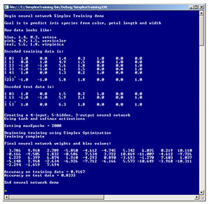
Take a look at the demo program in Figure 1. The demo program creates a neural network that predicts the species of an iris flower ("setosa," "versicolor" or "virginica") based on the flower's color (blue, pink or teal), petal length, and petal width. The demo uses 24 training items where non-numeric predictor color and non-numeric dependent variable species have been encoded.
 [Click on image for larger view.]
Figure 1. Neural Network Training Using Simplex Optimization
[Click on image for larger view.]
Figure 1. Neural Network Training Using Simplex Optimization
The first training item is { 1, 0, 1.4, 0.3, 1, 0, 0 }, which means a blue flower with length 1.4 and width 0.3 is the setosa species. The leading (1, 0) represents color blue. Colors pink and teal are encoded as (0,1) and (-1, -1), respectively. This is called 1-of-(N-1) encoding. The trailing (1, 0, 0) represents species setosa. Species versicolor and virginica are encoded as (0, 1, 0) and (0, 0, 1), respectively. This is called 1-of-N encoding.
The demo creates a 4-5-3 neural network to accommodate the four input values and the three output values. The choice of five for the number of hidden nodes was determined by trial and error. The demo uses simplex optimization with a maximum number of training iterations set to 2,000.
After training completed, the demo displayed the values of the 43 weights and biases, then computed the predictive accuracy of the model. For the 24-item training data, the neural network correctly predicted the species with 91.67 percent (22 out of 24) accuracy. For the six-item test data, the model predicted with 83.33 percent (5 out of 6) accuracy. This 83.33 percent value can be interpreted as a rough estimate of how well the model would predict if presented with iris flowers where the true value of the species isn't known.
This article assumes you have at least intermediate-level developer skills and a basic understanding of neural networks, but does not assume you know anything about simplex optimization. The demo program is coded in C# but you shouldn't have too much trouble refactoring the demo code to another .NET language.
Understanding Simplex Optimization
A simplex is a mathematical term for a triangle. The idea behind simplex optimization is to start with three possible solutions that can be thought of as the corners of a triangle. One possible solution will be "best" (meaning smallest error between computed and known output values), a second will be "worst" (largest error), and the third is called "other." Simplex optimization creates three new candidate solutions called "expanded," "reflected," and "contracted." Each of these candidates is compared against the current worst solution, and if any of the candidates is better (smaller error) than the current worst solution, the worst solution is replaced by the candidate.
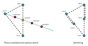
Simplex optimization is illustrated in Figure 2. In a simple case where a solution consists of two values, like (1.23, 4.56), you can think of a solution as a point on the (x, y) plane. The left side of Figure 2 shows how three new candidate solutions are generated from the current best, worst and "other" solutions.
 [Click on image for larger view.]
Figure 2. Simplex Optimization in Two Dimensions
[Click on image for larger view.]
Figure 2. Simplex Optimization in Two Dimensions
First, a centroid is computed. The centroid is the average of the best and "other" solutions. In two dimensions this is a point half-way between the "other" and best points. Next, an imaginary line is created, which starts at the worst point and extends through the centroid. The contracted candidate solution is between the worst and centroid points. The reflected candidate is on the imaginary line, past the centroid. And the expanded candidate is past the reflected point.
In each iteration of simplex optimization, if one of the expanded, reflected or contracted candidates is better than the current worst solution, worst is replaced by that candidate. But if none of the three candidates generated are better than the worst solution, the current worst and "other" solutions shrink toward the best solution to points somewhere between their current position and the best solution as shown in the right-hand side of Figure 2.
After each iteration, a new virtual "best-other-worst" triangle is formed, getting closer and closer to an optimal solution. If you imagine taking a snapshot of each triangle over time, when looked at sequentially, the moving triangles resemble a pointy blob moving across the surface in a way that resembles a single-celled amoeba. For this reason, simplex optimization is sometimes called amoeba method optimization.
There are many variations of simplex optimization, which vary in how far the contracted, reflected, and expanded candidate solutions are from the current centroid, and the order in which the candidate solutions are checked to see if each is better than the current worst solution. The most common form of simplex optimization is called the Nelder-Mead algorithm. The demo program uses a simpler variation, which doesn't have a specific name.
In high-level pseudo-code, the variation of simplex optimization used in the demo program is:
initialize best, worst, other solutions to random positions
loop maxEpochs times
  create centroid from worst and other
  create expanded
  if expanded is better than worst, replace worst with expanded,
    continue loop
  create reflected
  if reflected  is better than worst, replace worst with reflected,
    continue loop
  create contracted
  if contracted  is better than worst, replace worst with contracted,
    continue loop
  create a random solution
  if  random solution is better than worst, replace worst,
    continue loop
  shrink worst and other towards best
end loop
return best solution found
Simplex optimization, like all other machine learning optimization algorithms, has pros and cons. Compared to back-propagation, simplex optimization is easier to understand and modify, but it generally takes longer to generate good weight and bias values.
The Demo Program
To create the demo program, I launched Visual Studio and selected the C# console application program template and named it SimplexTraining. The demo has no significant Microsoft .NET Framework version dependencies, so any relatively recent version of Visual Studio should work. After the template code loaded, in the Solution Explorer window I renamed file Program.cs to SimplexProgram.cs and Visual Studio automatically renamed class Program.
The demo program is too long to present in its entirety in this article, but the entire source code is available in a code download accompanying this article. All normal error checking has been removed to keep the main ideas as clear as possible.
The demo code begins:
using System;
namespace SimplexTraining
{
  class SimplexProgram
  {
    static void Main(string[] args)
    {
      Console.WriteLine("\Begin Simplex Training demo\n");
      // Other messages here
      double[][] trainData = new double[24][];
      trainData[0] = new double[] { 1, 0, 1.4, 0.3, 1, 0, 0 };
      trainData[1] = new double[] { 0, 1, 4.9, 1.5, 0, 1, 0 };
      // And so on
      trainData[23] = new double[] { -1, -1, 5.8, 1.8, 0, 0, 1 };
...
The 24-item training data set is hardcoded for simplicity. In a non-demo scenario you'd likely read the data into memory from a text file. The data isn't normalized because all the magnitudes of the values are roughly the same so no variable will dominate the others. In a realistic environment you'll usually want to normalize your data. The demo data is artificial but is based on "Fisher's Iris Data," a well-known 150-item real benchmark data set.
Next, the six-item training data is set up:
double[][] testData = new double[6][];
testData[0] = new double[] { 1, 0, 1.5, 0.2, 1, 0, 0 };
testData[1] = new double[] { -1, -1, 5.9, 2.1, 0, 0, 1 };
testData[2] = new double[] { 0, 1, 1.4, 0.2, 1, 0, 0 };
testData[3] = new double[] { 0, 1, 4.7, 1.6, 0, 1, 0 };
testData[4] = new double[] { 1, 0, 4.6, 1.3, 0, 1, 0 };
testData[5] = new double[] { 1, 0, 6.3, 1.8, 0, 0, 1 };
In most cases all your data will be in one file and you would create the training and test data using a helper method named something like SplitData. After setting up the training and test data, the demo displays the data using program-defined helper method ShowData:
Console.WriteLine("Encoded training data is: \n");
ShowData(trainData, 5, 1, true);
Console.WriteLine("Encoded test data is: \n");
ShowData(testData, 2, 1, true);
Next, the demo instantiates a fully connected, feed-forward neural network:
Console.WriteLine("\nCreating a 4-input, 5-hidden, 3-output neural network");
Console.WriteLine("Using tanh and softmax activations \n");
int numInput = 4;
int numHidden = 5;
int numOutput = 3;
NeuralNetwork nn = new NeuralNetwork(numInput, numHidden, numOutput);
The neural network classifier uses hard-coded hyperbolic tangent and softmax activation functions. Parameterizing the activation functions would add more flexibility but at the cost of a significant increase in complexity.
The demo trains the neural network using this code:
int maxEpochs = 2000;
Console.WriteLine("Setting maxEpochs = " + maxEpochs);
Console.WriteLine("\nBeginning training using Simplex Optimization");
double[] bestWeights = nn.Train(trainData, maxEpochs);
Console.WriteLine("Training complete \n");
Console.WriteLine("Final neural network weights and bias values:");
ShowVector(bestWeights, 10, 3, true);
The demo concludes by displaying the best weights and bias values found, and computing the model's accuracy:
...
  nn.SetWeights(bestWeights);
  double trainAcc = nn.Accuracy(trainData);
  Console.WriteLine("\nAccuracy on training data = " +
    trainAcc.ToString("F4"));
  double testAcc = nn.Accuracy(testData);
  Console.WriteLine("Accuracy on test data = " +
    testAcc.ToString("F4"));
  Console.WriteLine("\nEnd neural network demo\n");
  Console.ReadLine();
} // Main
In a realistic scenario, the model weights and bias values would be saved to file so they could be used to make predictions for new, previously unseen iris flowers.
The Training Method
The demo program consists of a Program class that houses the Main method, and a NeuralNetwork class that defines a neural network object. The heart of simplex optimization is contained in class method Train. The definition of method Train begins:
public double[] Train(double[][] trainData, int maxEpochs)
{
  Solution[] solutions = new Solution[3]; // Best, worst, other
  // Initialize three solutions to random values
  int numWeights = (numInput * numHidden) + numHidden +
    (numHidden * numOutput) + numOutput;
  for (int i = 0; i < 3; ++i)
  {
    solutions[i] = new Solution(numWeights);
    solutions[i].weights = RandomSolutionWts(numWeights);
    solutions[i].error =
      MeanSquaredError(trainData, solutions[i].weights);
  }
...
The demo program uses a helper class named Solution. Recall that simplex optimization maintains best, worst and other solutions. This means that the three solutions must be sorted from smallest error to largest error. Therefore it's useful to define a Solution class that inherits from the IComparable interface so that an array of Solution objects can be automatically sorted by error, using the built-in Array.Sort method.
The definition of class Solution is presented in Listing 1. For simplicity, the weights and error fields are declared with public scope.
Listing 1: The Solution Class
private class Solution : IComparable<Solution>
{
  public double[] weights; // a potential solution
  public double error;     // MSE of weights

  public Solution(int numWeights)
  {
    this.weights = new double[numWeights]; // problem dim + constant
    this.error = 0.0;
  }

  public int CompareTo(Solution other) // low-to-high error
  {
    if (this.error < other.error)
      return -1;
    else if (this.error > other.error)
      return 1;
    else
      return 0;
  }
} // Solution
The demo program defines class Solution inside class NeuralNetwork. An alternative design is to define class Solution as a standalone class. The weights for each of the three solutions are supplied by helper method RandomSolutionWts, which is defined:
private double[] RandomSolutionWts(int numWeights)
{
  double[] result = new double[numWeights];
  double lo = -10.0;
  double hi = 10.0;
  for (int i = 0; i < result.Length; ++i)
    result[i] = (hi - lo) * rnd.NextDouble() + lo;
  return result;
}
The method restricts all weight and bias values to between -10.0 and +10.0 to help avoid model over-fitting. After creating an array of three Solution objects, method Train prepares the main algorithm loop:
int best = 0; // For solutions[idx].error
int other = 1;
int worst = 2;

int epoch = 0;
while (epoch < maxEpochs)
{
  ++epoch;
  // Simplex algorithm here
}
Local variables best, other, and worst act as indices into the array of solutions and are more descriptive than literals 0, 1, and 2. The main loop exits after maxEpochs iterations. An alternative is to add an early exit condition if Solution objects best and worst get very close to each other, indicating that training has converged and isn't likely to change anymore.
Inside the main loop, after incrementing the epoch counter variable, the three current simplex solutions are determined, and the centroid is computed:
Array.Sort(solutions); // [0] = best
double[] bestWts = solutions[0].weights;
double[] otherWts = solutions[1].weights;
double[] worstWts = solutions[2].weights;
double[] centroidWts = CentroidWts(otherWts, bestWts);
Recall that the centroid is the average of the best solution and the other solution. Helper method CentroidWts is defined:
private double[] CentroidWts(double[] otherWts, double[] bestWts)
{
  int numWeights = otherWts.Length;
  double[] result = new double[numWeights];
  for (int i = 0; i < result.Length; ++i)
    result[i] = (otherWts[i] + bestWts[i]) / 2.0;
  return result;
}
After creating the current centroid, method Train computes the expanded candidate and checks to see if it's better than the current worst point:
double[] expandedWts = ExpandedWts(centroidWts, worstWts);
double expandedError = MeanSquaredError(trainData, expandedWts);
if (expandedError < solutions[worst].error) // Better than worst?
{
  Array.Copy(expandedWts, worstWts, expandedWts.Length); // Replace
  solutions[worst].error = expandedError;
  continue;
}
Helper method ExpandedWts is defined:
private double[] ExpandedWts(double[] centroidWts, double[] worstWts)
{
  int numWeights = centroidWts.Length;
  double gamma = 2.0; // How far from centroid
  double[] result = new double[numWeights];
  for (int i = 0; i < result.Length; ++i)
    result[i] = centroidWts[i] + (gamma * (centroidWts[i] - worstWts[i]));
  return result;
}
Local variable gamma controls how far the expanded point is from the centroid. Larger values of gamma allow greater jumps and, therefore, faster training, at the risk of hopping over a good solution. If the expanded point isn't better than the current worst point, a reflected candidate is tried:
double[] reflectedWts = ReflectedWts(centroidWts, worstWts);
double reflectedError = MeanSquaredError(trainData, reflectedWts);
if (reflectedError < solutions[worst].error) // Better than worst?
{
  Array.Copy(reflectedWts, worstWts, reflectedWts.Length);
  solutions[worst].error = reflectedError;
  continue;
}
If the reflected candidate isn't better than the worst solution, a contracted candidate is tried:
double[] contractedWts = ContractedWts(centroidWts, worstWts);
double contractedError = MeanSquaredError(trainData, contractedWts);
if (contractedError < solutions[worst].error) // Better than worst?
{
  Array.Copy(contractedWts, worstWts, contractedWts.Length);
  solutions[worst].error = contractedError;
  continue;
}
Next, a random solution is tried:
double[] randomSolWts = RandomSolutionWts(numWeights);
double randomSolError = MeanSquaredError(trainData, randomSolWts);
if (randomSolError < solutions[worst].error)
{
  Array.Copy(randomSolWts, worstWts, randomSolWts.Length);
  solutions[worst].error = randomSolError;
  continue;
}
Instead of trying a random solution whenever the expanded, reflected and contracted candidates aren't better than the current worst solution, because it's expensive to evaluate a candidate, you may want to only try a random solution every 10 or 100 iterations.
At this point, no improvement was found, so the simplex shrinks:
...
  for (int j = 0; j < numWeights; ++j)
    worstWts[j] = (worstWts[j] + bestWts[j]) / 2.0;
  solutions[worst].error = MeanSquaredError(trainData, worstWts);

  for (int j = 0; j < numWeights; ++j)
    otherWts[j] = (otherWts[j] + bestWts[j]) / 2.0;
  solutions[other].error = MeanSquaredError(trainData, otherWts);
} // While
Finally, after maxEpochs attempts, the main loop terminates:
…
  this.SetWeights(solutions[best].weights);
  return solutions[best].weights;
} // Train
The best neural network weights and bias values found will be stored in array solutions[0], so these values are copied into the neural network's weights and bias values using class member method SetWeights. For convenience, a reference to the best weights is also returned. You might want to return the best weights and bias values by value rather than by reference.
Wrapping Up
The code and explanation presented in this article should give you a solid foundation for understanding and experimenting with neural network training using simplex optimization. The demo code has many customization points and room for performance improvements. That said, however, I've successfully used the code in this article on several real-world classification problems. As a general rule of thumb, when training a neural network, I usually try back propagation and simplex optimization, as well as particle swarm optimization. No one training method works best in all problem scenarios.