The Data Science Lab
Fundamentals of T-Test Using R
Linear regression was easy, right? Now, let's check out t-test analysis using R.
The R system consists of a scripting language, an interactive command shell and a large library of mathematical functions that can be used for data analysis. Although R has been around for many years, interest in R among software developers has increased significantly over the past couple of years, perhaps in part because R has been adopted by Microsoft as part of its technology stack.
One of the most fundamental types of R analysis is the t-test. In most cases the t-test is used when you want to compare the means (averages) of two groups in situations where you only have samples of the two groups under investigation.
The basic scenario is best explained by example. Imagine that you work for a very large school and want to investigate the difference in mathematical ability of the male students in a certain grade versus the female students. Because the math ability exam is time-consuming and expensive, you can't give the exam to all of the students. So you randomly select a sample of the males and a sample of the females and administer the exam to the two groups.
The t-test calculates the mean score of each of the two samples and compares the two sample means to infer if the two means of the parent populations (all male students and all female students) are probably the same or not.
The basic scenario is sometimes called a two independent samples t-test. In addition to the basic scenario, the t-test can be used to investigate if the mean of some group is equal to a constant value or not (called a one sample t-test). And the t-test can be used in before-and-after and similar scenarios. For example, suppose you give the math exam to a randomly selected group of students (both male and female) and record their scores. Then you administer some sort of training, and retest the same students. You can use the t-test to infer if the training had a positive effect -- that is, if the mean score after taking the training is greater than the mean score before taking the training. This is called a paired t-test.
T-Test for Two Independent Samples
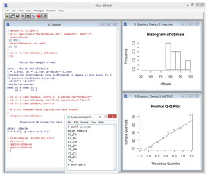
Take a look at the sample R session in Figure 1. The goal of the session is to investigate the math ability of a group of males versus a group of females. You can imagine that a math exam is given to 10 randomly selected males and 10 randomly selected females. Suppose the source data is stored in a text file named MaleFemale.txt in directory C:\TTest. The contents of the data file look like:
# math scores
male,female
85,78
82,84
. . .
88,83
76,
# end data
 [Click on image for larger view.]
Figure 1. T-Test Using R
[Click on image for larger view.]
Figure 1. T-Test Using R
In R, the "#" character is the default token to indicate the start of a comment. The data is comma-delimited and has a header line. There are eight scores for males and seven scores for females -- two males and three females did not complete the exam for some reason.
I installed R from r-project.org. The installation process is quick and painless. I installed version 3.1.2, but the t-test has no version dependencies so any relatively recent version of R will work for you. After installation, I launched an R environment by double-clicking on file Rgui.exe at C:\Program Files\R\R-3.1.2\bin\x64.
I cleared the console display by entering a Ctrl+L command. The demo R session begins with these two commands:
> setwd("C:\\TTest")
> d <- read.table("MaleFemale.txt", header=T, sep=",")
The first command sets the working directory to the location of the source data file. The second command can be interpreted to mean, "Use the read.table function to store into a data frame object named d, the contents of file MaleFemale.txt where the file has a header line and data items are separated by the comma character." You can think of an R data frame as being somewhat similar to an ADO.NET DataTable object.
The next two session commands and associated responses are:
> mean(d$male)
[1] 83.5
> mean(d$female, na.rm=T)
[1] 78
The first command is an instruction to calculate the average of the values in the "male" column of the d object. The result is 83.5. The second command calculates the average of the "female" column with a notation to remove (ignore) NA (missing) values.
The next two commands perform the t-test:
> t1 <- t.test(d$male, d$female)
> t1
The first command means, "Store into an object named t1, the results of a t-test on the values in the 'male' and 'female' columns of the data frame object d." The second command means, "Display the object named t1."
The output of the t-test begins with a title, "Welch Two Sample t-test." There are actually several different variations of the t-test. The original version is often called Student's t-test. The R t.test function uses an improved version called the Welch t-test.
The key output line of the t-test is:
t = 1.4062, df = 12.059, p-value = 0.1849
Of the three values, the most important is the p-value. The p-value is the probability that the two parent population means are equal. This is called the null hypothesis. Specifically, here the p-value is the probability that the true average math score for all males in the target group is equal to the true average math score for all females.
You can see all the available field names of an R object using the attributes function, for example, by entering the command attributes(t1). The value of a particular field can be accessed using the '$' qualifier, for example, by entering the command t1$p.value.
Interpreting the results of almost any statistical test, including the t-test, is very subtle, and usually more difficult than actually performing the test. Here, the p-value is 0.1849, or a bit less than 20 percent. You'd be inclined to reason that because the p-value is quite small, means the probability that the average score of all males is equal to the average score of all females is quite small, and therefore conclude that the true mean scores of males and females do in fact differ. And this is a completely reasonable conclusion.
However, it is customary to use a threshold probability value of 0.05 (or sometimes 0.01) for a conclusion. The threshold value is called the significance level. So a more common interpretation of this result would be something along the lines of, "Even though the p-value is quite small, it's not smaller than a significance level of 0.05. Therefore, I won't reject the null hypothesis that the means of the two groups are the same, and I conclude there's not quite strong enough evidence to indicate that the means of the two groups are different." Expressed tersely, the conclusion is, "I do not reject the null hypothesis that the means are equal."
One Sample T-Tests
The demo R session in Figure 1 performs three one sample t-tests:
> t2 <- t.test(d$male, mu=85.0, alternative="greater")
> t3 <- t.test(d$female, mu=76.0, alternative="less")
> t4 <- t.test(d$male, mu=85.0)
The first command means, "Store into an object named t2, the results of a t-test to see if the true mean of all male students is greater than 85." The parameter mu is so-named because Greek letter mu (which resembles a lowercase "u") is the math symbol for a mean. To save space I didn't display the results. A very small p-value would indicate that the true mean math score of all males is equal to 85 and, therefore, the mean is not greater than 85. The larger the p-value, the more likely it is that the true mean is in fact greater than 85.
The second command is a test to infer if the true mean math score of all female students is less than 76. A small p-value would indicate that the true mean is equal to 76, so the larger the p-value is, the more likely it is that the true mean is less than 76.
The third command is a test to infer if the true mean of all male students is equal to 85. A small p-value would indicate that the true mean is 85 and the larger the p-value is, the more likely the true mean is not equal to 85. In the call to the t-test I could've explicitly specified the default value of the alternative parameter, which is "two.sided" rather than "equal" or "equals," as you might have guessed.
T-Test Assumption of Normality
All variations of the t-test, including the Welch variation, assume that the two parent populations (or the single parent population in the case of a one sample test) are normally, or Gaussian, distributed. So in principle, before even performing a t-test you should examine the sample values to see if there's any indication that the populations from which they're drawn are not normal. But in practice the assumption is usually examined after performing the t-test.
There are many R techniques to check the t-test assumption of population normality. The demo session in Figure 1 uses three common techniques, two of which I recommend and one technique I do not recommend. The first approach in the demo session uses the Shapiro-Wilk test. The command that tests the normality of the scores of the male students is:
> shapiro.test(d$male)
The output is:
W = 0.955, p-value = 0.7612
The p-value is the probability that the parent population is normal. This relatively large result, 0.7612, indicates that the true mean score of all males is close to normal. You could repeat this test for the female scores, too. Even though it's quite common, I do not recommend using the Shapiro-Wilk test because in my opinion the results are usually ambiguous with regard to the t-test assumption of normality.
The demo R session tests the population normality assumption using two visual techniques. The first approach is to simply plot the sample data and use an eyeball test to see if the resulting graphs are roughly bell shaped. The command to plot the male scores is:
> hist(d$male, xlim=c(50,100))
This means, "Draw a histogram (bar chart) of the values in the male column of the d data frame, where the x-axis ranges from 50 to 100." If you examine the histogram in Figure 1 you can see that it doesn't look normal at all. However, because there are so few data points, you could conclude the male scores are close enough to normal for the t-test to be valid.
The second visual technique is to construct what's called a quantile-quantile plot. The commands to plot the male scores are:
> dev.new()
> qqnorm(d$male)
> qqline(d$male)
The dev.new function creates a new graphics window so that the histogram won't be overwritten. The qqnorm function creates the quantile-quantile plot and the qqline function adds a straight line to the plot. If the parent population is exactly normal, all the data points will lie exactly on the straight line in the quantile-quantile plot. Here, most of the data points are close to the line, so again you could conclude that the male scores, even though not exactly normal, are close enough to normal for the t-test to be valid.
To summarize, the t-test assumes that the parent populations are normally distributed. In most situations it's not practical to verify this assumption rigorously. I recommend using the hist and the qqnorm functions to perform a visual inspection of the sample data in order to confirm that the data isn't wildly un-normal.
Paired Sample T-Tests
Consider a data file named BeforeAfter.txt that has contents:
before,after
70,72
83,85
. . .
90,91
Each row represents the math exam scores of a student before and after some type of training. The pairs of data points are conceptually related, so a paired sample t-test is called for. The data could be loaded into memory like so:
> dd <- read.table("BeforeAfter.txt", header=T, sep=",")
Presumably, you'd want to see if the training improved scores; in other words, the mean of the "before" scores is less than the mean of the "after" scores. Your expectation is sometimes called a research hypothesis to distinguish it from the mathematical null hypothesis. An R command to perform a paired t-test is:
> t5 <- t.test(dd$before, dd$after, alternative="less", paired=T)
Compared to other forms of the t-test, the only real difference in the t.test function call is the addition of the paired=T argument. Typical output from an R paired t-test is:
> t5
Paired t-test
data:  dd$before and dd$after
t = -2.3772, df = 9, p-value = 0.02071
The p-value is the probability that the true mean of the population before-scores is equal to the true mean of the after-scores. In this example, the p-value of 0.02 is quite low, so you'd conclude that the mean before and mean after-scores are not the same and, therefore, the mean of the before-scores is in fact less than the mean of the after-scores and, therefore, the training was effective.
The value of t = -2.3772, and the value of df = 9 ("degrees of freedom") are used behind the scenes by the R t.test function to compute the p-value. In a college statistics class you'd dive into the meaning of t and df in great detail, but from a software developer's point of view, they're not critically important in most situations.
Parting Comments
As you've seen, it's relatively simple to know when a t-test is applicable and how to perform a t-test using R. However, interpreting the results of a t-test is a very delicate process. It's important to remember that the t-test is probabilistic and applies to groups, not individual items. My colleagues and I who work with statistics are often dismayed by completely incorrect causation conclusions drawn from statistics.
For example, suppose some t-test analysis of the annual salaries of two groups of people (say, males and females, or those over age 40 and those under 40) in a particular industry (say, software development) suggests that the mean salary of one group is less than the mean salary of the other group. This probabilistic result in no way suggests any reason why the group with the lower mean salary has a lower mean salary.
About the Author
Dr. James McCaffrey directs the data science and research efforts at Quaetrix, a data analytics company located near Redmond, Washington. Before joining Quaetrix, James was a senior research engineer at Microsoft. James can be reached at [email protected].