The Data Science Lab
Neural Network Batch Training Using Python
Our resident data scientist explains how to train neural networks with two popular variations of the back-propagation technique: batch and online.
Training a neural network is the process of determining the values of the constants -- called weights and biases -- that essentially define the network. You do this by using training data that has known correct output values and then finding values for the weights and biases that minimize the error between computed output values and the target values in the training data.
There are several techniques you can use to train a neural network. By far the most common is called back-propagation. Back-propagation has three main variations: batch, online and mini-batch. In this article I'll demonstrate how to train a neural network using both batch and online training. I'll address mini-batch training, which is a bit more complicated, in a future article.
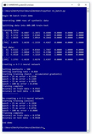
The best way to see where this article is headed is to take a look at the screenshot of a demo run in Figure 1 and the associated graph in Figure 2. The demo begins by generating 1,000 synthetic data items. One line of synthetic data looks like:
0.7779 -0.4087 -2.3072 0.4800 0 0 1
 [Click on image for larger view.]
Figure 1. Neural Network Batch Training in Action
[Click on image for larger view.]
Figure 1. Neural Network Batch Training in Action
 [Click on image for larger view.]
Figure 2. Batch vs. Online Training
[Click on image for larger view.]
Figure 2. Batch vs. Online Training
Each item has four features (predictor variables) with random values between -9.0 and +9.0, and three output values that are either (1, 0, 0), (0, 1, 0) or (0, 0, 1). The output values correspond to a classification problem where there are three possible labels to predict, such as (red, yellow, green).
After the 1,000-item synthetic data is created, it’s randomly split into 800 lines of training data and 200 lines of test data. The test data is held out during training and then used to evaluate the predictive accuracy of the trained neural network model.
The demo program creates a neural network with four input nodes, seven hidden processing nodes and three output nodes. The number of input and output nodes is determined by the structure of the data, but the number of hidden nodes is a free parameter and must be determined by trial and error in a non-demo scenario. Here, the value of seven is arbitrary.
The demo first trains the neural network using batch training. Training is an iterative process, and the demo uses 100 iterations. During training, an error is printed every 25 epochs (iterations). After the batch training has completed, the resulting model correctly predicts 94.00 percent of the test data (188 out of 200 correct).
Next, the demo resets the 4-7-3 neural network and trains using the online approach. After training completes, the resulting model correctly predicts 95.50 percent of the test data (191 out of 200 correct). So, for this example, batch training is slightly worse than online training.
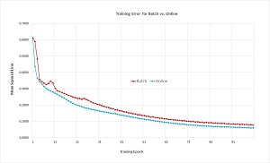
The graph in Figure 2 shows the error for both training approaches. Although a training error is a bit difficult to interpret, it appears that batch training is slightly worse than online training and is slightly more volatile, too. In fact, neural network batch training usually performs slightly worse than online training. But there are at least three good reasons why understanding batch training is important. First, there are times where batch training is better than online training (although you can only determine this by trial and error). Second, batch training is the basis of mini-batch training, which is the most common form of training (at least among my colleagues). Third, there are training algorithms other than back-propagation, such as swarm optimization, which use a batch approach.
The demo program is coded using Python. Although Python is too slow for complex neural networks, it's a good choice for relatively simple problems. Additionally, Python is the language of choice when using neural network code libraries such as Microsoft CNTK and Google TensorFlow, so understanding the demo Python code will help you use these code libraries more effectively. And coding a neural network from scratch gives you a code base for experimentation.
This article assumes you have a good knowledge of the neural network input-output mechanism, and intermediate or better programming skill with a C-family language (C#, Python, Java) but doesn’t assume you know much about the back-propagation algorithm or batch training. The demo program is too long to present in its entirety in this article, but the complete source code is available in the accompanying download.
Batch and Online Back-Propagation
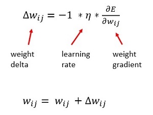
Batch and online training are variations of the back-propagation training algorithm. In each iteration of the algorithm, each weight and bias is updated by adding a delta value, which can be either positive or negative. A neural network bias is a special kind of weight, and for the remainder of this article I refer to both as just weights. The basic weight update equations, expressed using math symbols, are shown in Figure 3. Expressed using pseudo-code, a weight delta is delta[i,j] = -1 * lr * grad(w[i,j]) and a weight update is w[i,j] = w[i,j] + delta.
 [Click on image for larger view.]
Figure 3. Basic Back-Propagation Update Equations
[Click on image for larger view.]
Figure 3. Basic Back-Propagation Update Equations
There is a weight value connecting each pair of input and hidden nodes, and each pair of hidden and output nodes. Weights are just values, typically between -10.0 and +10.0. The i and j are indices that indicate a pair of weights. For a given set of input and output values and known target values, each weight has an associated gradient value (a calculus derivative) that indicates how to adjust the weight so that the computed output values will move closer to the target values.
The lr in pseudo-code (Greek eta in the math equation -- looks like lower case script "n") is the learning rate, which is a small constant, typically a value between about 0.01 and 0.20. Suppose during training, one of the neural network weights is 5.00 and for a training item, the associated gradient is -0.20. If the learning rate is set to 0.10, then the weight delta is -1 * 0.10 * -0.20 = 0.02, and so the new weight value would be 5.00 + 0.02 = 5.02. The -1 constant in the weight delta is there only so that each weight is updated by adding -- rather than subtracting -- its associated delta.
Batch and online training differ slightly in how the weight gradients are calculated and when the weights are updated. In pseudo-code, online back-propagation training for a single training epoch is:
<li>loop each training item
  compute output values
  for-each weight
    use target and output to compute gradient
  end-for
  for-each weight
    use gradient to compute weight delta
    use delta to update weight
  end-for
end-loop</li>
Notice that in online training, each weight is updated based on the computed output results of a single training item. In pseudo-code, batch online training for a single training epoch is:
<li>loop each training item
  compute output values
  for-each weight
    use target and output to compute gradient
    accumulate gradient value
  end-for
end-loop
for-each weight
  use accumulated gradient to compute delta
  use delta to update weight
end-for</li>
The key difference in batch training is that each weight update is based on an accumulated gradient that in turn is based on the results of all training items. Put another way, batch training updates a weight based on all available gradient information, but online training uses a single training item to essentially estimate the total gradient.
In the early days of neural networks, batch training was generally favored over online training because it seemed like a more logical approach. However, in practice, online training usually gave better results. A common compromise approach is called mini-batch training. In mini-batch training, instead of processing a single training item to estimate the overall gradient -- or processing all training items to compute a weight gradient -- you process chunks of training items. For example, in the demo where there are 800 training items, you might process 160 items (20 percent) at a time. Although simple in principle, implementing mini-batch training is somewhat tricky, as I’ll explain in a future column.
Overall Demo Program Structure
The overall demo program structure, with a few minor edits to save space, is presented in Listing 1. To edit the demo program, I used Notepad. Most of my colleagues prefer using one of the many nice Python editors available.
I commented the name of the program and indicated the Python version used. I added three import statements to gain access to the NumPy package's array and matrix data structures, and the math and random modules.
Listing 1: Overall Program Structure
# nn_batch.py
# Python 3.x

import numpy as np
import random
import math

# helper functions

def makeData(numFeatures, numHidden, numClasses,
  numRows, nn_seed):
def splitData(data, trainPct):
def showVector(v, dec):
def showMatrixPartial(m, numRows, dec, indices):

class NeuralNetwork:

def main():
  print("\nBegin NN batch train demo \n")

  numRows = 1000
  print("Generating " + str(numRows) + " rows of data ")
  allData = makeData(4, 5, 3, numRows, nn_seed=1)
  print("Splitting data into 80%-20% train-test \n")
  (trainData, testData) = splitData(allData, trainPct=0.80)
  print("Training data: ")
  showMatrixPartial(trainData, 3, 4, True)
  print("\nTest data: ")
  showMatrixPartial(testData, 3, 4, True)

  numInput = 4
  numHidden = 7
  numOutput = 3
  print("\nCreating a %d-%d-%d neural network " %
    (numInput, numHidden, numOutput) )
  nn = NeuralNetwork(numInput, numHidden, numOutput,
    seed=13)

  maxEpochs = 100
  learnRate = 0.01
  print("\nSetting maxEpochs = " + str(maxEpochs))
  print("Setting learning rate = %0.3f " % learnRate)

  print("Starting training (batch)")
  nn.trainBatch(trainData, maxEpochs, learnRate)
  print("Training complete")

  accTrain = nn.accuracy(trainData)
  accTest = nn.accuracy(testData)

  print("Accuracy on train data = %0.4f " % accTrain)
  print("Accuracy on test data  = %0.4f " % accTest)

  print("-------------")

  print("\nRe-creating a %d-%d-%d neural network " %
    (numInput, numHidden, numOutput) )
  nn = NeuralNetwork(numInput, numHidden, numOutput,
    seed=13)

  learnRate = 0.01  # not necessarily optimum

  print("Starting training (online)")
  nn.trainOnline(trainData, maxEpochs, learnRate)
  print("Training complete")

  accTrain = nn.accuracy(trainData)
  accTest = nn.accuracy(testData)

  print("Accuracy on train data = %0.4f " % accTrain)
  print("Accuracy on test data  = %0.4f " % accTest)

  print("\nEnd demo ")

if __name__ == "__main__":
  main()

# end script
The demo program consists mostly of a program-defined NeuralNetwork class. I created a main function to hold all program control logic. The demo begins by generating synthetic data:
def main():
  print("\nBegin NN batch train demo \n")

  numRows = 1000
  print("Generating " + str(numRows) + " rows of data ")
  allData = makeData(4, 5, 3, numRows, nn_seed=1)
...
The makeData function creates a local 4-5-3 neural network with random weight and bias values, then generates random input values and computes output. Next, the demo splits the 1,000 items into a training matrix (80 percent of the data) and a test matrix:
print("Splitting data into 80%-20% train-test \n")
(trainData, testData) = splitData(allData, trainPct=0.80)
print("Training data: ")
showMatrixPartial(trainData, 3, 4, True)
print("\nTest data: ")
showMatrixPartial(testData, 3, 4, True)
The splitData function returns the two matrices in a two-item tuple, and displays the matrices using helper function showMatrixPartial. Next, the demo creates a neural network to model the training data:
numInput = 4
numHidden = 7
numOutput = 3
print("\nCreating a %d-%d-%d neural network " %
  (numInput, numHidden, numOutput) )
nn = NeuralNetwork(numInput, numHidden, numOutput,
  seed=13)
Notice the training network has the same number of input (4) and output (3) nodes as the neural network used to generate the synthetic data, in order to match the structure of the data. But the training network has a different number of hidden nodes (7 instead of 5) and a different random seed for weight initialization, because using the same number of hidden nodes and seeds would make training the network a bit too easy.
The demo performs batch training like so:
maxEpochs = 100
learnRate = 0.01
nn.trainBatch(trainData, maxEpochs, learnRate)
accTrain = nn.accuracy(trainData)
accTest = nn.accuracy(testData)
print("Accuracy on train data = %0.4f " % accTrain)
print("Accuracy on test data  = %0.4f " % accTest)
The NeuralNetwork class defines two different training methods: trainBatch and trainOnline. This is a simple approach at the expense of some redundant code in the two methods.
The demo concludes by performing online training:
nn = NeuralNetwork(numInput, numHidden, numOutput,
  seed=13)
learnRate = 0.01  # not necessarily optimum
nn.trainOnline(trainData, maxEpochs, learnRate)
accTrain = nn.accuracy(trainData)
accTest = nn.accuracy(testData)
print("Accuracy on train data = %0.4f " % accTrain)
print("Accuracy on test data  = %0.4f " % accTest)
I re-instantiated the neural network because, otherwise, the online training would be starting with a fully trained network. I used the same learning rate, 0.01, but because online and batch training compute the weight gradients in different ways, it's possible that a single learning rate value could favor one technique over the other.
The Batch Training Method
The trainBatch method of the program-defined NeuralNetwork class is quite complex. The method has local arrays and matrices to hold the accumulated gradients:
while epoch < maxEpochs:
  ihWtsAccGrads = np.zeros(shape=[self.ni, self.nh],
    dtype=np.float32)  # accumulated input-to-hidden
  hBiasesAccGrads = np.zeros(shape=[self.nh],
    dtype=np.float32)  # accumulated hidden biases
  hoWtsAccGrads = np.zeros(shape=[self.nh, self.no],
    dtype=np.float32)  # accumulated hidden-to-output
  oBiasesAccGrads = np.zeros(shape=[self.no],
    dtype=np.float32)  # accumulated output biases
When performing online training you should visit each training item in scrambled order so the algorithm doesn't get stuck in an oscillating mode. But when doing batch training, because the gradients are accumulated over all training items, you don't need to scramble the order in which items are visited:
for ii in range(numTrainItems):  # visit each item
  idx = indices[ii]  # not scrambled
Each gradient is accumulated. For example, the input-to-hidden weight gradients are computed then accumulated like so:
for i in range(self.ni):
  for j in range(self.nh):
    ihGrads[i,j] = hSignals[j] * self.iNodes[i]
    ihWtsAccGrads[i,j] += ihGrads[i,j]
The code is a bit more complicated than it first appears because a lot of work is done computing the so-called hidden node signals, which isn’t shown. After all training items have been visited, weights are updated. For example, the input-to-hidden weight are updated with this code:
for i in range(self.ni):
  for j in range(self.nh):
    delta = -1.0 * learnRate * ihWtsAccGrads[i,j]
    self.ihWeights[i,j] += delta
Notice that batch training and online training require about the same amount of computation, but the number of weight updates is different. Loosely, for batch training, each weight is updated maxEpochs times (using a full gradient that requires numTrain calculations). For online training, each weight is updated maxEpochs * numTrain times (using an estimated gradient that requires one calculation).
Wrapping Up
In the early days of neural networks, there was quite a bit of controversy about which training technique, batch or online, was preferable. As computer processing power increased, the difference became less important. For simple neural networks, most of my colleagues try online training first, then, if results aren’t satisfactory, they'll try batch or mini-batch training. Like many machine learning activities, there are very few rules of thumb and a bit of experimentation is usually needed.
Once you understand the differences between batch and online training, you're in a good position to understand the strengths and weaknesses of the compromise mini-batch training technique. For complex neural networks, mini-batch training is usually the default approach used by my colleagues.