The Data Science Lab
Neural Network L1 Regularization Using Python
The data science doctor continues his exploration of techniques used to reduce the likelihood of model overfitting, caused by training a neural network for too many iterations.
Regularization is a technique used to reduce the likelihood of neural network model overfitting. Model overfitting can occur when you train a neural network for too many iterations. This sometimes results in a situation where the trained neural network model predicts the output values for the training data very well, with little error and high accuracy, but when the trained model is applied to new, previously unseen data, the model predicts poorly.
There are several forms of regularization. The two most common forms are called L1 and L2 regularization. This article focuses on L1 regularization, but I'll discuss L2 regularization briefly.
You can think of a neural network as a complex math function that makes predictions. Training is the process of finding values for the network weights and bias constants that effectively define the behavior of the network. The most common way to train a neural network is to use a set of training data with known input values and known, correct output values. You apply an optimization algorithm, typically back-propagation, to find weights and bias values that minimize some error metric between the computed output values and the correct output values (typically squared error or cross entropy error).
Overfitting is often characterized by weights that have large magnitudes, such as +38.5087 and -23.182, rather than small magnitudes such as +1.650 and -3.043. L1 regularization reduces the possibility of overfitting by keeping the values of the weights and biases small.
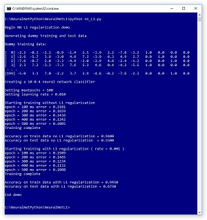
A good way to see where this article is headed is to take a look at the screenshot of a demo program in Figure 1. The demo program is coded using raw Python (no libraries) with the NumPy numeric library, but you should have no trouble refactoring to another language, such as C# or Visual Basic, if you want.
 [Click on image for larger view.] Neural Network L1 Regularization Demo Program
The demo begins by using a utility neural network to generate 200 synthetic training items and 40 test items. Each data item has 10 input predictor variables (often called features) and four output variables (often called class labels) that represent 1-of-N encoded categorical data. For example, if you were trying to predict the political leaning of a person, and there are just four possible leanings, you could encode conservative as (1, 0, 0, 0), moderate as (0, 1, 0, 0), liberal as (0, 0, 1, 0) and radical as (0, 0, 0, 1).
The demo program creates a neural network classifier with 10 input nodes, eight hidden processing nodes and four output nodes. The number of input and output nodes is determined by the data, but the number of hidden nodes is a free parameter and must be determined by trial and error. The demo program trains a first model using the back-propagation algorithm without L1 regularization. That first model gives 94.00 percent accuracy on the training data (188 of 200 correct) and a poor 55.00 percent accuracy on the test data (just 22 of 40 correct). It appears that the model might be overfitted. To be honest, in order to get a demo result that illustrates typical regularization behavior, I cheated a bit by setting the number of training iterations to a small value (500), and the model is actually underfitted -- not trained enough.
The demo continues by training a second model, this time with L1 regularization. The second model gives 94.50 percent accuracy on the training data (189 of 200 correct) and 67.50 percent accuracy on the test data (27 of 40 correct). In this example, using L1 regularization has made a significant improvement in classification accuracy on the test data.
Understanding Neural Network Model Overfitting
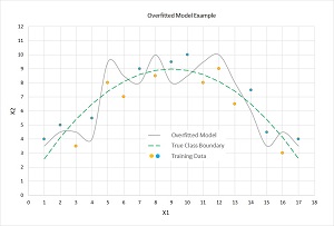
Model overfitting is often a significant problem when training a neural network. The idea is illustrated in the graph in Figure 2. There are two predictor variables: X1 and X2. There are two possible categorical classes, indicated by the orange (class = 0) and blue (class = 1) dots. You can imagine this corresponds to the problem of predicting if a loan application should be approved (1) or denied (0), based on normalized income (X1) and normalized debt (X2). For example, the left-most data point at (X1 = 1, X2 = 4) is colored blue (approve).
 [Click on image for larger view.] Neural Network Overfitting Example
The dashed green line represents the actual boundary between the two classes. This boundary is unknown to you. Notice that data items that are above the green line are mostly blue (7 of 9 points) and that data items below the green line are mostly orange (6 of 8 points). The four misclassifications in the training data are due to randomness inherent in almost all real-life data.
A good neural network model would find the true decision boundary represented by the dashed green line. However, if you train a neural network model too long, it will essentially get too good and produce a model indicated by the solid wavy gray line. Notice that the gray line makes perfect predictions on the test data: All the blue dots are above the gray line and all the orange dots are below the gray line.
However, when the overfitted model is presented with new, previously unseen data, there's a good chance the model will make an incorrect prediction. For example, a new data item at (X1 = 11, X2 = 9) is above the green dashed truth boundary and so should be classified as blue. But because the data item is below the gray line overfitted boundary, it will be incorrectly classified as orange.
If you vaguely remember your high school algebra you might recall that the overfitted gray line, with its peaky shape, looks like the graph of a polynomial function that has coefficients with large magnitudes. These coefficients correspond to neural network weights and biases. Therefore, the idea behind L1 regularization is to keep the magnitudes of the weights and bias values small, which will prevent a spikey decision boundary, which in turn will avoid model overfitting.
Understanding L1 Regularization
In a nutshell, L1 regularization works by adding a term to the error function used by the training algorithm. The additional term penalizes large-magnitude weight values. By far the two most common error functions used in neural network training are squared error and cross entropy error. For the rest of this article I'll assume squared error, but the ideas are exactly the same when using cross entropy error.
For L1 regularization, the weight penalty term that's added to the error term is a small fraction (often given the Greek letter lowercase lambda) of the sum of the absolute values of the weights. For example, suppose you have a neural network with only three weights. If you set lambda = 0.10 (actual values of the L1 constant are usually much smaller), and if the current values of the weights are (6.0, -2.0, 4.0) then in addition to the base squared error between computed output values and correct target output values, the augmented error term adds 0.10 * [ abs(6.0) + abs(-2.0) + abs(4.0) ] = 0.10 * (6.0 + 2.0 + 4.0) = 0.10 * 12.0 = 1.20 to the overall error.
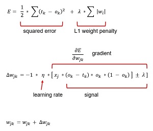
The key math equations (somewhat simplified for clarity) are shown in Figure 3. The bottom-most equation is the weight update for a weight connecting a hidden node j to an output node k. In words, "The new weight value is the old weight value plus a delta value."
 [Click on image for larger view.] L1 Regularization Equations
An example line of code in the demo is:
self.hoWeights[j,k] += delta
The top-most equation is a squared error with an L1 penalty term. In words, "Take each target value (tk), subtract the computed output value (ok), square the difference, add all the sums, and divide by 2, then add a small constant lambda times the sum of the absolute values of the weights."
The middle equation shows how a weight delta is calculated, assuming a squared error with L1 weight penalty. Overall, a delta is -1 times a small learning rate constant (Greek eta, which looks like lowercase script "n") times the gradient of the error function. The gradient is the Calculus derivative of the error function. The error function has two parts, the basic error plus the weight penalty. The derivative of a sum is the sum of the derivatives. The derivative of the left part of the error term is quite tricky and outside the scope of this article, but you can see it uses target values, computed output values and hidden node values (the xj).
To use L1 regularization, you need the Calculus derivative of weight penalty as part of the error term. As it turns out, if a weight is positive, then the derivative of the absolute value is just the constant +1 times lambda. If a weight is negative, the derivative is -1 times lambda. The absolute value function doesn't have a derivative at 0, but this isn't a problem. If a weight is 0, you can ignore the weight penalty term. The idea here is that the goal of L1 regularization is to keep the magnitudes of the weight values small. If a weight is 0, its magnitude can't get any smaller. An example from the demo is:
if self.hoWeights[j,k] > 0.0:
  hoGrads[j,k] += lamda
elif self.hoWeights[j,k] < 0.0:="" hograds[j,k]="" -="">
Put a bit differently, during training, the back-propagation algorithm iteratively adds a weight-delta (which can be positive or negative) to each weight. The weight-delta is a fraction of the weight gradient. The weight gradient is the Calculus derivative of the error function plus or minus the L1 regularization constant.
Implementing L1 Regularization
The overall structure of the demo program, with a few edits to save space, is presented in Listing 1.
Listing 1: L1 Regularization Demo Program Structure
# nn_L1.py
# Python 3.x

import numpy as np
import random
import math

# helper functions
def showVector(): ...
def showMatrixPartial(): ...
def makeData(): ...

class NeuralNetwork: ...

def main():
  print("Begin NN L1 regularization demo")

  print("Generating dummy training and test data")
  genNN = NeuralNetwork(10, 15, 4, 0)
  genNumWts = NeuralNetwork.totalWeights(10,15,4)
  genWeights = np.zeros(shape=[genNumWts], \
    dtype=np.float32)
  genRnd = random.Random(3)  # 3
  genWtHi = 9.9; genWtLo = -9.9
  for i in range(genNumWts):
    genWeights[i] = (genWtHi - genWtLo) * \
      genRnd.random() + genWtLo
  genNN.setWeights(genWeights)

  dummyTrainData = makeData(genNN, numRows=200, \
    inputsSeed=16)
  dummyTestData = makeData(genNN, 40, 18)
  print("Dummy training data: ")
  showMatrixPartial(dummyTrainData, 4, 1, True)

  numInput = 10
  numHidden = 8
  numOutput = 4
  print("Creating neural network classifier")
  nn = NeuralNetwork(numInput, numHidden, numOutput, seed=0)

  maxEpochs = 500
  learnRate = 0.01
  print("Setting maxEpochs = " + str(maxEpochs))
  print("Setting learning rate =  percent0.3f "  percent learnRate)

  print("Starting training without L1 regularization")
  nn.train(dummyTrainData, maxEpochs, learnRate)  # no L1
  print("Training complete")

  accTrain = nn.accuracy(dummyTrainData)
  accTest = nn.accuracy(dummyTestData)

  print("Accuracy on train data no L1 =  percent0.4f "  percent accTrain)
  print("Accuracy on test data no L1 =  percent0.4f "  percent accTest)

  L1_rate = 0.001
  nn = NeuralNetwork(numInput, numHidden, numOutput, seed=0)
  print("Starting training with L1 regularization)
  nn.train(dummyTrainData, maxEpochs, learnRate, \
    L1=True, lamda=L1_rate)
  print("Training complete")

  accTrain = nn.accuracy(dummyTrainData)
  accTest = nn.accuracy(dummyTestData)

  print("Accuracy on train data with L1 =  percent0.4f "  percent accTrain)
  print("Accuracy on test data with L1 =  percent0.4f "  percent accTest)

  print("\nEnd demo \n")

if __name__ == "__main__":
  main()

# end script


Most of the demo code is a basic feed-forward neural network implemented using raw Python. The key code that adds the L1 penalty to each of the hidden-to-output weight gradients is:

for j in range(self.nh):  # each hidden node
  for k in range(self.no):  # each output
    hoGrads[j,k] = oSignals[k] * self.hNodes[j]
    if L1 == True:
      if self.hoWeights[j,k] > 0.0:
        hoGrads[j,k] += lamda
      elif self.hoWeights[j,k] < 0.0:="" hograds[j,k]="" -="">
The hoGrads matrix holds hidden-to-output gradients. First, each base gradient is computed as the product of the associated output node signal and the associated input, which is a hidden node value. The computation of the output node signals isn't shown. Then, if the Boolean L1 flag parameter is set to True, an additional lambda parameter value (spelled as "lamda" to avoid a clash with the Python language keyword) is either added or subtracted, depending on the sign of the associated weight.
The input-to-hidden weight gradients are computed similarly:
for i in range(self.ni):
  for j in range(self.nh):
    ihGrads[i, j] = hSignals[j] * self.iNodes[i]
    if L1 == True:
      if self.ihWeights[i,j] > 0.0:
        ihGrads[i,j] += lamda
      elif self.ihWeights[i,j] < 0.0:="" ihgrads[i,j]="" -="lamda">
After using L1 regularization to compute modified gradients, the weights are updated exactly as they would be without L1. For example:
# update input-to-hidden weights
for i in range(self.ni):
  for j in range(self.nh):
    delta = learnRate * ihGrads[i,j]
    self.ihWeights[i,j] += delta
Somewhat surprisingly, it's normal practice to not apply the L1 penalty to the hidden node biases or the output node biases. The reasoning is rather subtle, but briefly and informally, a single bias value with large magnitude isn't likely to lead to model overfitting because a large bias value can be compensated for by the multiple associated weights.
An Alternative Approach to L1
If you review how L1 regularization works, you'll see that on each training iteration, each weight is decayed toward zero by a small, constant value. The weight decay toward zero may or may not be counteracted by the non-penalty part of the weight gradient. The approach presented in this article follows the theoretical definition of L1 regularization where the weight penalty is part of the underlying error term, and is therefore part of the weight gradient. The weight delta is a small constant times the gradient.
An alternative approach, which simulates theoretical L1 regularization, is to compute the gradient as normal, without a weight penalty term, and then tack on an additional value that will move the current weight closer to zero.
For example, suppose a weight has value 8.0 and you're training with a learning rate = 0.05 and an L1 lambda value = 0.01. Suppose the weight gradient, without the L1 term, is 9.0. Then, using the theoretical approach presented in this article, the weight delta = -1 * 0.05 * (9.0 + 0.01) = -0.4505 and the new value of the weight is 8.0 - 0.4505 = 7.5495.
But if you use the tack-on approach, the weight delta is -1 * (0.05 * 9.0) = -0.4500 and the new value of the weight is 8.0 - 0.4500 - 0.01 = 7.5400. The point is that when you're using a neural network library, such as Microsoft CNTK or Google TensorFlow, exactly how L1 regularization is implemented can vary. This means an L1 lambda that works well with one library may not work well with a different library if the L1 implementations are different.
Wrapping Up
The other common form of neural network regularization is called L2 regularization. L2 regularization is very similar to L1 regularization, but with L2, instead of decaying each weight by a constant value, each weight is decayed by a small proportion of its current value. In many scenarios, using L1 regularization drives some neural network weights to 0, leading to a sparse network. Using L2 regularization often drives all weights to small values, but few weights completely to 0. I covered L2 regularization more thoroughly in a previous column, aptly
named "Neural Network L2 Regularization Using Python."
There are very few guidelines about which form of regularization, L1 or L2, is preferable. As is often the case with neural network training, trial and error must be used. That said, L2 regularization is slightly more common than L1, mostly because L2 usually, but not always, works better than L1. It is possible to use both L1 and L2 together. This is called an elastic network.
Finally, recall that the purpose of L1 regularization is to reduce the likelihood of model overfitting. There are other techniques that have the same purpose, including node dropout, jittering, train-validate-test early stopping and max-norm constraints.