The Data Science Lab
Naive Bayes Classification Using Python
Naive Bayes classification is a machine learning technique that can be used to predict the class of an item based on two or more categorical predictor variables. For example, you might want to predict the grender (0 = male, 1 = female) of a person based on occupation, eye color and nationality.
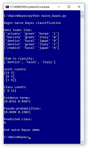
A good way to see where this article is headed is to look at the screenshot of a demo run in Figure 1 and the associated data (with indexes added for readability) in Listing 1. The demo program uses a dummy data file of 20 items. Each item represents a person's occupation (actuary, barista, chemist, dentist), eye color (green, hazel), and nationality (Italy, Japan, Korea). The value to predict is encoded as 0 or 1, which makes this a binary classification problem; however, naive Bayes can handle multiclass problems with three or more values.
 [Click on image for larger view.]
Figure 1. Naive Bayes Classification Demo Run
[Click on image for larger view.]
Figure 1. Naive Bayes Classification Demo Run
The demo predicts the class of a person with (occupation, eye color, nationality) attributes of (dentist, hazel, italy). Behind the scenes, the demo scans the data and computes six joint counts. The items that have both dentist and class 0 are at indexes [2], [14] and [15]. Each joint count is incremented by one so that no joint count is zero. Therefore, the joint count for dentist and class 0 is 3 + 1 = 4. Similarly, the other five incremented joint counts are: dentist and 1 = 5, hazel and 0 = 6, hazel and 1 = 2, italy and 0 = 3, and italy and 1 = 6. The demo also counts and displays the raw number (not incremented) of items for each class. There are 8 items that are class 0 and 12 items that are class 1.
Listing 1: Dummy Data with Indexes Added
 0 actuary green korea 1
 1 barista green italy 0
 2 dentist hazel japan 0
 3 dentist green italy 1
 4 chemist hazel japan 0
 5 actuary green japan 1
 6 actuary hazel japan 0
 7 chemist green italy 1
 8 chemist green italy 1
 9 dentist green japan 1
10 barista hazel japan 0
11 dentist green japan 1
12 dentist green japan 1
13 chemist green italy 1
14 dentist green japan 0
15 dentist hazel japan 0
16 chemist green korea 1
17 barista green japan 1
18 actuary hazel italy 1
19 actuary green italy 0
The demo uses the joint count and class count information to compute intermediate values called evidence terms. There is one evidence term for each class. Then the evidence terms are used to compute pseudo-probabilities for each class. In the demo, the pseudo-probabilities are (0.6698, 0.3302) and because the first value is largest the predicted class is 0.
This article assumes you have intermediate or better programming skill with Python or a C-family language but doesn't assume you know anything about naive Bayes classification. The complete demo code and the associated data are presented in this article and in an attached zip file download.
How Naive Bayes Works
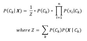
The math for naive Bayes is quite deep, but implementation is relatively simple. The key math equation is shown in Figure 2. In words, the equation is, "The probability that a class is k given predictor values X is one over Z times the probability of class k, times the product of the probabilities of each x given class k." This equation is best explained by example.
 [Click on image for larger view.]
Figure 2. The Key Math Equation for Naive Bayes
[Click on image for larger view.]
Figure 2. The Key Math Equation for Naive Bayes
The first step is to scan though the source data and compute joint counts. If there are nx predictor variables (three in the demo) and nc classes (two in the demo), then there are nx * nc joint counts to compute.
After calculating joint counts, 1 is added to each count. This is called Laplacian smoothing and is done to prevent any joint count from being 0, which would zero-out the final results. For the demo data the smoothed joint counts are:
dentist and 0:  3 + 1 = 4
dentist and 1:  4 + 1 = 5
hazel and 0:    5 + 1 = 6
hazel and 1:    1 + 1 = 2
italy and 0:    2 + 1 = 3
italy and 1:    5 + 1 = 6
Next, the raw counts of class 0 items and class 1 items are computed. Because these counts will always be greater than zero, no smoothing factor is needed. For the demo data the class counts are:
class 0:   8
class 1:  12
Next, an evidence term for each class is calculated. For class 0 the evidence term is:
Z(0) = (4 / 8+3) * (6 / 8+3) * (3 / 8+3) * (8 / 20)
        = 4/11 * 6/11 * 3/11 * 8/20
        = 0.3636 * 0.5455 * 0.2727 * 0.4
        = 0.0216
The first three terms of calculation for Z(0) uses the smoothed joint counts for class 0, divided by the class count for 0 (8) plus the number of predictor variables (nx = 3) to compensate for the three additions of 1 due to the Laplacian smoothing. The fourth term is the probability of class 0. The calculation of the class 1 evidence term follows the same pattern:
 Z(1) = (5 / 12+3) * (2 / 12+3) * (6 / 12+3) * (12 / 20)
        = 5/15 * 2/15 * 6/15 * 12/20
        = 0.3333 * 0.1333 * 0.4000 * 0.6
        = 0.0107
The last step is to compute pseudo-probabilities:
P(class 0) = Z(0) / (Z(0) + Z(1))
                 = 0.0216 / (0.0216 + 0.0107)
                 = 0.6698

P(class 1) = Z(1) / (Z(0) + Z(1))
                 = 0.0107 / (0.0216 + 0.0107)
                 = 0.3302
The denominator sum is called the evidence and is used to normalize the evidence terms so that they sum to 1.0 and can be loosely interpreted as probabilities. Notice that if you just want to make a prediction, you can use the largest evidence term and skip the normalization step.
The Demo Program
The complete demo program, with a few minor edits to save space, is presented in Listing 2. I used the awesome Notepad to edit my program but most of my colleagues prefer a more sophisticated editor such as Visual Studio Code. I indent with two spaces instead of the usual four to save space.
Listing 2: The Naive Bayes Demo Program
# naive_bayes.py
# Python 3.6.5
import numpy as np

def main():
  print("Begin naive Bayes classification ")
  data = np.loadtxt(".\\people_data_20.txt",
    dtype=np.str, delimiter=" ")
  print("Data looks like: ")
  for i in range(5):
    print(data[i])
  print(". . . \n")

  nx = 3  # number predictor variables
  nc = 2  # number classes
  N = 20  # data items

  joint_cts = np.zeros((nx,nc), dtype=np.int)
  y_cts = np.zeros(nc, dtype=np.int)

  X = ['dentist', 'hazel', 'italy']
  print("Item to classify: ")
  print(X)

  for i in range(N):
    y = int(data[i][nx])  # class in last column
    y_cts[y] += 1
    for j in range(nx):
      if data[i][j] == X[j]:
        joint_cts[j][y] += 1

  joint_cts += 1  # Laplacian smoothing

  print("\nJoint counts: ")
  print(joint_cts)
  print("\nClass counts: ")
  print(y_cts)

  # compute evidence terms using log trick
  e_terms = np.zeros(nc, dtype=np.float32)
  for k in range(nc):
    v = 0.0
    for j in range(nx):
      v += np.log(joint_cts[j][k]) - np.log(y_cts[k] + nx)
    v += np.log(y_cts[k]) - np.log(N)
    e_terms[k] = np.exp(v)

  np.set_printoptions(4)
  print("\nEvidence terms: ")
  print(e_terms)

  evidence = np.sum(e_terms)
  probs = np.zeros(nc, dtype=np.float32)
  for k in range(nc):
    probs[k] = e_terms[k] / evidence

  print("\nPseudo-probabilities: ")
  print(probs)

  pc = np.argmax(probs)
  print("\nPredicted class: ")
  print(pc)

  print("\nEnd naive Bayes demo ")

if __name__ == "__main__":
  main()
All normal error-checking has been omitted to keep the main ideas as clear as possible. To create the data file, I used Notepad and copy-pasted the 20 data items shown in Listing 1 and removed the indexes. I named the data file as people_data_20.txt and saved it in the same directory as the demo program.
Loading Data into Memory
The demo program loads the data into memory as an array-of-arrays NumPy matrix named data like so:
data = np.loadtxt(".\\people_data_20.txt",
  dtype=np.str, delimiter=" ")
print("Data looks like: ")
for i in range(5):
  print(data[i])
print(". . . \n")
Each field in the demo data is delimited with a single blank space character. You might want to use tab characters instead. If you have the indexes in the data file you can either read them into memory and then ignore them, or you can use the usecols parameter of the loadtxt() function to strip the indexes away.
There are several different types of naive Bayes classification. The type used in the demo requires all predictor values to be categorical so that they can be counted. A different type of naive Bayes classification can handle numeric predictor values, but in my opinion naive Bayes is best suited for strictly categorical data. If you do have data with numeric values, you can bin the data into categories such as (low, medium, high), and use the technique presented in this article.
Computing the Evidence Terms
The joint counts and raw class counts are computed by these statements:
joint_cts = np.zeros((nx,nc), dtype=np.int)
y_cts = np.zeros(nc, dtype=np.int)
for i in range(N):
  y = int(data[i][nx])  # class in last column
  y_cts[y] += 1
  for j in range(nx):
    if data[i][j] == X[j]:
      joint_cts[j][y] += 1
joint_cts += 1  # Laplacian smoothing
The code assumes the class value is the last item in the data file and is therefore the last column in the matrix holding the data. Adding 1 to each joint count applies the aforementioned Laplacian smoothing.
A direct computation of the evidence terms would look like:
for k in range(nc):
  v = 1.0
  for j in range(nx):
    v *= joint_cts[j][k] / (y_cts[k] + nx)
Notice that an evidence term is the product of several values that are less than 1.0 and you could easily run into an arithmetic underflow problem. The demo program uses what is sometimes called the log trick:
e_terms = np.zeros(nc, dtype=np.float32)
for k in range(nc):
  v = 0.0
  for j in range(nx):
    v += np.log(joint_cts[j][k]) - np.log(y_cts[k] + nx)
  v += np.log(y_cts[k]) - np.log(N)
  e_terms[k] = np.exp(v)
The key idea is that log(A * B) = log(A) + log(B) and log(A / B) = log(A) - log(B). So, by using the log of each count, you can add and subtract many small values instead of multiplying and dividing. Applying the exp() function to the result of log operations restores the correct result.
Wrapping Up
The "naive" part of the term naive Bayes classification refers to the fact that the technique assumes all the predictor variables are mathematically independent of one another. This is almost never true, but in practice naive Bayes classification often works quite well. A common strategy is to use naive Bayes together with a second classification technique such as logistic regression. You perform each classification separately then compute a consensus prediction. Such combined techniques are common in machine learning and are called ensemble methods.
About the Author
Dr. James McCaffrey directs the data science and research efforts at Quaetrix, a data analytics company located near Redmond, Washington. Before joining Quaetrix, James was a senior research engineer at Microsoft. James can be reached at [email protected].