The Data Science Lab
How To Code Modern Neural Networks Using Python and NumPy
Although neural networks have been studied for decades, over the past couple of years there have been many small but significant changes in the default techniques used. For example, ReLU (rectified liner unit) hidden node activation is now the most common form of hidden layer activation for deep neural networks, and the Glorot weight initialization technique has largely replaced the uniform random technique.
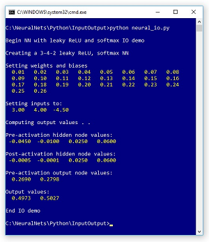
In this article, and in future Data Science Lab articles, I'll present and explain the most common modern techniques used for neural networks. A good way to see where this article is headed is to examine the screenshot of a demo program in Figure 1.
The demo program illustrates the neural network input-output mechanism for network with a single hidden layer, leaky ReLU hidden layer activation, and softmax output layer activation. The demo creates a neural network with 3 input nodes, 4 hidden nodes, and 2 output nodes.
The 3-4-2 network has 26 weights and biases which are initialized to dummy values of 0.01 through 0.26. Input values (3.0, 4.0, -4.5) are sent to the network and the computed output values are (0.4973, 0.5027).
 [Click on image for larger view.]
Figure 1. Neural Network IO Demo Program
[Click on image for larger view.]
Figure 1. Neural Network IO Demo Program
This article assumes you have a basic familiarity with Python or a C-family language such as C# or JavaScript, but doesn't assume you know anything about neural networks. The demo program is a bit too long to present in its entirety in this article, but the complete source code is available in the accompanying file download.
I wrote the demo using the 3.6.5 version of Python and the 1.14.3 version of NumPy but any relatively recent versions will work fine. It's possible to install Python and NumPy separately, however, if you're new to Python and NumPy I recommend installing the Anaconda distribution of Python which simplifies installation and gives you many additional useful packages.
Understanding Neural Network Input-Output
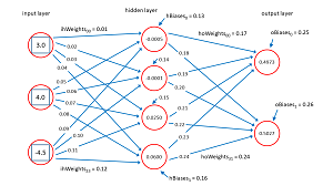
Before looking at the demo code, it's important to understand the neural network input-output mechanism. The diagram in Figure 2 corresponds to the demo program.
 [Click on image for larger view.]
Figure 2.Neural Network Input-Output
[Click on image for larger view.]
Figure 2.Neural Network Input-Output
The input node values are (3.0, 4.0, -4.5). Each line connecting input-to-hidden and hidden-to-output nodes represents a numeric constant called a weight. If nodes are zero-based indexed with node [0] at the top of the diagram, then the weight from input[0] to hidden[0] is 0.01 and the weight from hidden[3] to output[1] is 0.24.
Each hidden node and each output node (but not the input nodes) has an additional special weight called a bias. The bias value for hidden[3] is 0.16 and the bias for output[0] is 0.25.
Notice that if there are ni input nodes and nh hidden nodes and no output nodes then there are a total of (ni * nh) + nh + (nh * no) + no weights and biases. For the demo 3-4-2 neural net there are (3 * 4) +4 + (4 * 2) + 2 = 26 weights and bias values.
In words, to compute the value of a hidden node, you multiply each input value times its associated input-to-hidden weight, add the products up, then add the bias value, and then apply the leaky ReLU function to the sum.
The leaky ReLU function is very simple. In code:
def leaky(x):
  if x <= 0.0:
    return 0.01 * x
  else:
    return x
For example, leaky(1.234) = 1.234 and leaky(-2.34) = 0.01 * -2.34 = -0.0234. The plain ReLU function returns 0.0 instead of 0.01 * x when x <= 0.0:
def relu(x):
  if x <= 0.0:
    return 0.0
  else:
    return x
Both functions have similar performance but in my experience, leaky ReLU usually works a bit better for neural networks with a single hidden layer.
The calculation for hidden node [0] is:
h_sum[0] = (3.0)(0.01) + (4.0)(0.05) + (-4.5)(0.09) + 0.13
                = -0.0450

hidden[0] = leaky(-0.0450)
                = -0.00045
The ReLU and leaky ReLU functions were created specifically for deep neural networks to reduce the likelihood of pathological behavior called the vanishing gradient problem. However, ReLU and its variations seem to work quite well for simple networks too. The older hyperbolic tangent and logistic sigmoid functions are still quite common for simple networks. For example:
def log_sig(x):
  if x < -20.0:
    return 0.0
  elif x > 20.0:
    return 1.0
  else:
    return 1.0 / (1.0 + np.exp(-x))
The output nodes are calculated much like the hidden nodes but instead of using leaky ReLU, a special function called softmax is used for activation. The preliminary sum of products plus bias values of output nodes [0] and [1] are:
o_sum[0] = (-0.0005)(0.17) + (-0.0001)(0.19) + (0.0250)(0.21) + (0.0600)(0.23) + 0.25
                = 0.2690

o_sum[1] = (-0.0005)(0.18) + (-0.0001)(0.20) + (0.0250)(0.22) + (0.0600)(0.24) + 0.26
                = 0.2798
The softmax function is best explained by example:
divisor = exp(0.2690) +  exp(0.2798)
            = 1.3087 + 1.3229
            = 2.6315

output[0] = exp(0.2690) / 2.6315
               = 0.4973

ouput[1] = exp(0.2798) / 2.6315
              = 0.5027
Notice that softmax uses the exp(x) function which can be astronomically large for even moderate values of x. The demo program uses a clever algebra trick ("the softmax max trick") to reduce the possibility of arithmetic overflow.
The purpose of softmax activation is to scale output values so that they sum to 1.0 and can be interpreted as probabilities. Suppose the demo corresponded to a problem where the goal is to predict if a person is male or female based on three predictor variables such as annual income, years of education, and height. If male is encoded as (1, 0) and female is encode as (0, 1) then the prediction is female because the second output value (0.5027) is larger than the first (0.4973). Note: it's relatively uncommon to use (1, 0) and (0, 1) encoding for a binary classification problem, but I used this encoding in the explanation to match the demo neural network architecture.
Overall Program Structure
The overall program structure is presented in Listing 1. To edit the demo program I used the basic Notepad program. Most of my colleagues prefer using one of the many nice Python editors that are available. I indent with two spaces rather than the usual four.
I commented the name of the program and indicated the Python version used. I placed utility functions, such as show_vec() and leaky() in a file named my_utilities.py and placed that file in a directory named Utilities.
Listing 1: Overall Program Structure
# neural_io.py
# Python 3.6.5

import sys
sys.path.insert(0, "..\\Utilities")
import my_utilities as U

import numpy as np

# ------------------------------------

class NeuralNetwork: . . .

# ------------------------------------

def main():
  print("\nBegin NN with leaky ReLU IO demo ")

  # 1. create network
  print("\nCreating a 3-4-2 leaky ReLU, softmax NN")
  nn = NeuralNet(3, 4, 2)

  # 2. set weights and biases
  wts = np.array([0.01, 0.02, 0.03, 0.04, 0.05, 0.06,
    0.07, 0.08, 0.09, 0.10, 0.11, 0.12,  # ih weights
    0.13, 0.14, 0.15, 0.16,  # h biases
    0.17, 0.18, 0.19, 0.20,  # ho weights
    0.21, 0.22, 0.23, 0.24,
    0.25, 0.26], dtype=np.float32)  # o biases

  print("\nSetting weights and biases")
  U.show_vec(wts, wid=6, dec=2, vals_line=8)
  nn.set_weights(wts)

  # 3. set input
  X = np.array([3.0, 4.0, -4.5], dtype=np.float32)
  print("\nSetting inputs to: ")
  U.show_vec(X, 6, 2, len(X))

  # 4. compute outputs
  print("\nComputing output values . . ")
  Y = nn.eval(X)
  print("\nOutput values: ")
  U.show_vec(Y, 8, 4, len(Y))

  print("\nEnd IO demo ")

if __name__ == "__main__":
  main()
The demo program consists mostly of a program-defined NeuralNetwork class. I created a main function to hold all program control logic. I set up the demo neural network like so:
def main():
  print("\Begin NN with leaky ReLU and softmax IO demo ")
  # 1. create network
  print("\nCreating a 3-4-2 leaky ReLU, softmax NN")
  nn = NeuralNet(3, 4, 2)
. . .
The weights and bias values are set using these statements:
  # 2. set weights and biases
  wts = np.array([0.01, 0.02, 0.03, 0.04, 0.05, 0.06,
    0.07, 0.08, 0.09, 0.10, 0.11, 0.12,  # ih weights
    0.13, 0.14, 0.15, 0.16,  # h biases
    0.17, 0.18, 0.19, 0.20,  # ho weights
    0.21, 0.22, 0.23, 0.24,
    0.25, 0.26], dtype=np.float32)  # o biases

  print("\nSetting weights and biases")
  U.show_vec(wts, wid=6, dec=2, vals_line=8)
  nn.set_weights(wts)
All the weights and biases are placed in a single vector using the order input-hidden weights, followed by hidden biases, followed by hidden-output weights, followed by output biases.
The input values are prepared like this:
  # 3. set input
  X = np.array([3.0, 4.0, -4.5], dtype=np.float32)
  print("\nSetting inputs to: ")
  U.show_vec(X, 6, 2, len(X))
And then the output values are generated like so:
. . .
  # 4. compute outputs
  print("\nComputing output values . . ")
  Y = nn.eval(X)
  print("\nOutput values: ")
  U.show_vec(Y, 8, 4, len(Y))
  print("\nEnd IO demo ")
if __name__ == "__main__":
  main()
The eval() method implements the neural network input-output process described above.
The Neural Network Class
The neural network class has one constructor and three methods. The structure of the Python neural network class is:
class NeuralNetwork:
  def __init__(self, num_input, num_hidden, num_output): . . .
  def set_weights(self, weights): . . .
  def get_weights(self): . . .
  def eval(self, x_values): . . .
The __init__() function is the class constructor. Unlike many programming languages, in Python you do not have to declare a class member variable before referencing it inside the constructor. All class members have public scope.
The definition of the __init__() method begins with:
def __init__(self, num_input, num_hidden, num_output):
  self.ni = num_input
  self.nh = num_hidden
  self.no = num_output
. . .
Even though all class method definitions (except those marked as @staticmethod) must include the "self" parameter, when a class method is called, the "self" argument is not used. But when accessing a class method or variable, the "self" keyword with dot notation must precede all method and variable names.
Next, three NumPy vectors are created to hold the input, hidden, and output nodes:
self.i_nodes = np.zeros(shape=[self.ni], dtype=np.float32)
self.h_nodes = np.zeros(shape=[self.nh], dtype=np.float32)
self.o_nodes = np.zeros(shape=[self.no], dtype=np.float32)
The syntax should be interpretable by you if you have experience with a C-family language. The default data type for the NumPy zeros function is "float64" (equivalent to the C# type "double"). Specifying float32 is common for neural networks because 64-bit precision is rarely needed. Next, matrices for the node-to-node weights, and vectors for the node bias values are initialized:
self.ih_weights = np.zeros(shape=[self.ni,self.nh], dtype=np.float32)
self.ho_weights = np.zeros(shape=[self.nh,self.no], dtype=np.float32)
self.h_biases = np.zeros(shape=[self.nh], dtype=np.float32)
self.o_biases = np.zeros(shape=[self.no], dtype=np.float32)
For the ih_weights ("input-to-hidden") matrix, the first (row) index references an input node and the second (column) index references a hidden node. Similarly, the row index of ho_weights references a hidden node and the column index references an output node. For example, ho_weights[2,0] holds the weight that connects hidden node [2] with output node [0].
The __init__() method concludes with:
self.h_sums = np.zeros(shape=[self.nh], dtype=np.float32)
self.o_sums = np.zeros(shape=[self.no], dtype=np.float32)
These two vectors hold the pre-activation sum of weight times node products.
Computing Output Values
The input-output mechanism is implemented in class method eval(). The definition begins by computing the pre-activation hidden layer sum of products:
def eval(self, x_values):
  self.i_nodes = x_values  # by ref
  for j in range(self.nh):
    for i in range(self.ni):
      self.h_sums[j] += self.i_nodes[i] * self.ih_weights[i,j]
    self.h_sums[j] += self.h_biases[j]  # add the bias

  print("\nPre-activation hidden node values: ")
  U.show_vec(self.h_sums, 8, 4, len(self.h_sums))
. . .
The input nodes are copied by reference because they don't change. The call to show_vec() utility is just for demo purposes and wouldn't be used in most situations. If you're familiar with matrix multiplication, notice that the two for-loops that compute the hidden node sum of products are just unwound matrix multiplication. So the code could have been written using Python high-level constructions as:
self.h_sums = np.dot(self.i_nodes, self.ih_weights)
self.h_sums += self.h_biases
Next, leaky ReLU activation is applied to the hidden nodes sum of products:
for j in range(self.nh):
  self.h_nodes[j] = U.leaky(self.h_sums[j])

print("\nPost-activation hidden node values: ")
U.show_vec(self.h_nodes, 8, 4, len(self.h_sums))
After the values of the hidden nodes have been computed, they are used to compute the pre-softmax values of the output nodes:
for k in range(self.no):
  for j in range(self.nh):
    self.o_sums[k] += self.h_nodes[j] * self.ho_weights[j,k]
  self.o_sums[k] += self.o_biases[k]
print("\nPre-activation output node values: ")
U.show_vec(self.o_sums, 8, 4, len(self.o_sums))
The eval() method concludes by applying softmax activation:
softout = U.softmax(self.o_sums)
for k in range(self.no):
  self.o_nodes[k] = softout[k]

result = np.zeros(shape=self.no, dtype=np.float32)
for k in range(self.no):
  result[k] = self.o_nodes[k]

return result
Because the softmax function requires the values of all pre-activation output sum of products to compute a common divisor, it's more efficient to define a softmax implementation that operates on all pre-activation sums rather than on each individual sum. The implementation of function softmax in the utilities file uses the "max trick" to reduce the possibility of arithmetic overflow:
def softmax(vec):
  n = len(vec)
  result = np.zeros(n, dtype=np.float32)
  mx = np.max(vec)
  divisor = 0.0
  for k in range(n):
    divisor += np.exp(vec[k] - mx)
  for k in range(n):
    result[k] =  np.exp(vec[k] - mx) / divisor
  return result
The softmax function is an interesting topic in its own right, and you can find more information in the Wikipedia article on the function.
Wrapping Up
Python has been used for many years, and with the emergence of deep neural code libraries such as TensorFlow and PyTorch, Python is now clearly the language of choice for working with neural systems. Understanding how neural networks work at a low level is a practical skill for networks with a single hidden layer and will enable you to use deep neural network libraries more effectively.