The Data Science Lab
How to Create a Radial Basis Function Network Using C#
Dr. James McCaffrey of Microsoft Research explains how to design a radial basis function (RBF) network -- a software system similar to a single hidden layer neural network -- and describes how an RBF network computes its output.
A radial basis function (RBF) network is a software system that is similar to a single hidden layer neural network. In this article I explain how to design an RBF network and describe how an RBF network computes its output. I use the C# language but you shouldn't have any trouble refactoring the demo code to another programming language if you wish.
A good way to see where this article is headed is to take a look at the demo program shown in the screenshot in Figure 1. The demo sets up a 3-4-2 RBF network. There are three input nodes, four hidden nodes, and two output nodes. You can imagine that the RBF network corresponds to a problem where the goal is to predict if a person is male or female based on their age, annual income, and years of education.
The number of input nodes and number of output nodes in an RBF network are determined by the problem data, but the number of hidden nodes is a hyperparameter that must be determined by trial and error.
The demo program sets dummy values for the RBF network's centroids, widths, weights, and biases. The demo sets up a normalized input vector of (1.0, -2.0, 3.0) and sends it to the RBF network. The final computed output values are (0.0079, 0.9921). If the output nodes correspond to (0, 1) = male and (1, 0) = female, then you'd conclude that the person is male.
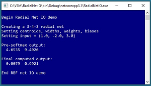 [Click on image for larger view.] Figure 1: RBF Network Input-Output Demo
This article assumes you have intermediate or better skill with C# but doesn’t assume you know anything about RBF networks. The code for demo program is a bit too long to present in its entirety in this article but the complete source code is available in the associated file download.
Understanding RBF Networks
The diagram in Figure 2 corresponds to the demo program. There are three input nodes with values (1.0, -2.0, 3.0). There are four hidden nodes. Each hidden node has a centroid which is a vector that has the same number of values as the input vector. A centroid is often given the symbol Greek lower case mu or English lower case u. In the diagram, u0 is (-3.0, -3.5, -3.8), u1 is (-1.0, -1.5, -1.8) and so on.
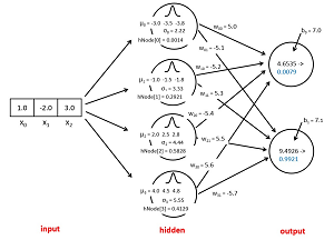 [Click on image for larger view.] Figure 2: The Demo RBF Network
Each hidden node also has a single width value. The width values are sometimes called standard deviations, and are often given the symbol Greek lower case sigma or lower case English s. In the diagram, s0 is 2.22, s1 is 3.33 and so on.
Each hidden node has a value which is determined by the input node values, and the hidden node's centroid values and the node's width value. In the diagram, the value of hidden node [0] is 0.0014, the value of hidden node [1] is 0.2921 and so on.
It is common to place a bell-shaped curve icon next to each hidden node in an RBF network diagram to indicate that the nodes are computed using a radial basis function with centroids and widths rather than using input-to-hidden weights as computed by single hidden layer neural networks.
There is a weight value associated with each hidden-to-output connection. The demo 3-4-2 RBF network has 4 * 2 = 8 weights. In the diagram, w00 is the weight from hidden [0] to output [0] and has value 5.0. Weight w01 is from hidden [0] to output [1] and has value -5.1 and so on.
There is a bias value associated with each output node. The bias associated with output [0] is 7.0 and the bias associated with output [1] is 7.1.
The two output node values of the demo RBF network are (0.0079, 0.9921). Notice the final output node values sum to 1.0 so that they can be interpreted as probabilities. Internally, the RBF network computes preliminary output values of (4.6535, 9.4926). These preliminary output values are then scaled so that they sum to 1.0 using the softmax function.
To recap, the output values of a 3-4-2 RBF network are determined by its 3 input values, the values of the 4 centroid vectors (each of which has 3 values), the 4 width values, the 4 * 2 = 8 weight values, and the 2 bias values. In the demo program the values of the centroids, widths, weights and biases are set to arbitrary dummy values. In a non-demo RBF network the values of the centroids, widths, weights and biases must be determined by training the network using data that has known correct input values and known correct output values.
The RBF Network Input-Output Mechanism
The first step in RBF network input-output is to compute the values of the hidden nodes. The math equation for the value of hidden node j is shown in Figure 3. In the equation, x is the input vector, e is Euler's number (approximately 2.71828), mu is the centroid vector associated with the hidden node, sigma is the associated width, and the set of double pipe characters is the norm (length) of a vector.
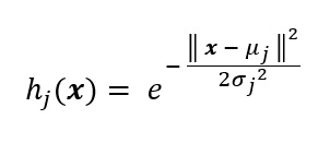 Figure 3: The Value of an RBF Network Hidden Node
The equation is a bit tricky and is perhaps best explained by a concrete example. Suppose x = (3, 7, 2), u = (1, 4, 2), and s = 1.5.
x – u = (3, 7, 2) – (1, 4, 2) = (2, 3, 0)
|| x – u || = sqrt( 2^2 + 3^2 + 0^2 ) = sqrt(13.0) = 3.61
|| x – u ||^2 = 13.0
-1 * || x – u ||^2 / 2s^2 = -13.0 / 2 * (1.5)^2 = -2.89
e^-2.89 = 0.0556
The difference of two vectors is a vector of the differences of the components. The norm of a vector is the square root of the sum of the squared components. The squared norm of a vector undoes the square root operation of the norm so the computation can be simplified by not performing the square root and squaring operations. Euler's number raised to a power is the exp() function which is available in almost all programming languages.
Another way to understand the radial basis function is to examine a standalone implementation:
public static double RadialBasis(double[] x,
  double[] u, double s)
{
  int n = x.Length;
  double sum = 0.0;
  for (int i = 0; i < n; ++i)
    sum += (x[i] - u[i]) * (x[i] - u[i]);
  return Math.Exp(-sum / (2 * s * s));
}
Such an implementation could be called like so:
double[] x = new double[] { 3, 7, 2 };
double[] u = new double[] { 1, 4, 2 };
double s = 1.5;
double rbf = RadialBasis(x, u, s);
Console.WriteLine(rbf);  // 0.0556
The result of a radial basis function applied to two vectors is a single value where smaller values indicate the two vectors are farther apart. For example, if the two vectors passed to an RBF function are identical, the function will return 1. (Note: the preceding two sentences have been edited from the original to correct mistakes.)
After the value of each hidden node has been computed, the next step is to compute the preliminary value of the output nodes. In words, the preliminary value of an output node is the sum of the products of each hidden node and its associated weight, plus the associated bias.
For the demo RBF network, the preliminary value of output[0] is 4.6535 and is computed as follows. The hidden node values are h[0] = 0.0014, h[1] = 0.2921, h[2] = 0.5828, h[3] = 0.4129. The weights for output[0] are w[0][0] = 5.0, w[1][0] = -5.2, w[2][0] = -5.4, w[3][0] = 5.6, and the associated bias is b[0] = 7.0 and therefore:
output[0] = (0.0014)(5.0) + (0.2921)(-5.2) +
                  (0.5828)(-5.4) + (0.4129)(5.6) + 7.0

               = 0.0070 + (-1.5189) + (-3.1471) + 2.3122 + 7.0

               = 4.6532
Similarly, the preliminary value of output[1] is computed as:
output[1] = (0.0014)(-5.1) + (0.2921)(5.3) +
                  (0.5828)(5.5) + (0.4129)(-5.7) + 7.1

               = (-0.0071) + 1.5481 + 3.2054 + (-2.3535) + 7.1

               = 9.4926
After the preliminary values of the output nodes have been computed, the last step is to apply the softmax function to compute the final output node values. In words, to compute the softmax of a set of values, you compute Euler's number e raised to each value (the exp() function) and then sum. The softmax of a value is e raised to the value, divided by the sum.
For the demo program:
exp(4.6532) = 104.92
exp(9.4926) = 13261.23

sum = 104.92 + 13261.23 = 13366.15

softmax(4.6532) = 104.92 / 13366.15 = 0.0079
softmax(9.4926) = 113261.23 / 13366.15 = 0.9921
A naive implementation of softmax is:
static double[] Softmax(double[] vec)
{
  int n = vec.Length;
  double[] result = new double[n];
  double sum = 0.0;
  for (int i = 0; i < n; ++i)
    result[i] = Math.Exp(vec[i]);
  for (int i = 0; i < n; ++i)
    sum += result[i];
  for (int i = 0; i < n; ++i)
    result[i] /= sum;
  return result;
}
Because the value of the exp(x) function can be huge for even moderate values of x, a naive implementation of softmax can easily throw an arithmetic exception. One way to greatly reduce the likelihood of an arithmetic error is to use what is called the max trick. The demo program has an implementation of softmax using the max trick. An explanation of the details of the max trick for the softmax function can be found here.
The Demo Program
To create the demo program, I launched Visual Studio 2019. I used the Community (free) edition but any relatively recent version of Visual Studio will work fine. From the main Visual Studio start window I selected the "Create a new project" option. Next, I selected C# from the Language dropdown control and Console from the Project Type dropdown, and then picked the "Console App (.NET Core)" item.
The code presented in this article will run as a .NET Core console application or as a .NET Framework application. Many of the newer Microsoft technologies, such as the ML.NET code library, specifically target the .NET Core framework so it makes sense to develop most new C# machine learning code in that environment.
I entered "RadialNetIO" as the Project Name, specified C:\VSM on my local machine as the Location (you can use any convenient directory), and checked the "Place solution and project in the same directory" box.
After the template code loaded into Visual Studio, at the top of the editor window I removed all using statements to unneeded namespaces, leaving just the reference to the top level System namespace. The demo needs no other assemblies and uses no external code libraries.
In the Solution Explorer window, I renamed file Program.cs to the more descriptive RadialNetIOProgram.cs and then in the editor window I renamed class Program to class RadialNetIOProgram to match the file name. The structure of the demo program, with a few minor edits to save space, is shown in Listing 1.
Listing 1. RBF Network Input-Output Demo Program
using System;
namespace RadialNetIO
{
  class RadialNetIOProgram
  {
    static void Main(string[] args)
    {
      Console.WriteLine("Begin demo");

      Console.WriteLine("Creating a 3-4-2 radial net");
      RadialNet rn = new RadialNet(3, 4, 2);

      double[][] centroids = new double[4][];
      centroids[0] = new double[] { -3.0, -3.5, -3.8 };
      centroids[1] = new double[] { -1.0, -1.5, -1.8 };
      centroids[2] = new double[] { 2.0, 2.5, 2.8 };
      centroids[3] = new double[] { 4.0, 4.5, 4.8 };

      double[] widths = new double[4] { 2.22, 3.33,
        4.44, 5.55 };

      double[][] weights = new double[4][];
      weights[0] = new double[2] { 5.0, -5.1 };
      weights[1] = new double[2] { -5.2, 5.3 };
      weights[2] = new double[2] { -5.4, 5.5 };
      weights[3] = new double[2] { 5.6, -5.7 };

      double[] biases = new double[2] { 7.0, 7.1 };

      Console.WriteLine("Setting centroids, widths," +
       " weights, biases");
      Console.WriteLine("Setting input = (1.0," +
       " -2.0, 3.0)");

      rn.SetCentroids(centroids);
      rn.SetWidths(widths);
      rn.SetWeights(weights);
      rn.SetBiases(biases);

      double[] xValues = new double[3] { 1.0, -2.0,
        3.0 };

      double[] yValues = rn.ComputeOutputs(xValues);
      Console.WriteLine("Final computed output: ");
      ShowVector(yValues, 4, 8);


      Console.WriteLine("End RBF net IO demo ");
      Console.ReadLine();
    }

    public static void ShowVector(double[] v,
      int dec, int w) { . . }
  }

  public class RadialNet { . . }

} // ns
All of the program logic is contained in the Main() method. Helper function ShowVector() displays a numeric vector using a specified number of digits after the decimal point.
The RBF network definition is contained in a class named RadialNet. All normal error checking has been removed to keep the main ideas as clear as possible.
The demo begins by creating an uninitialized RBF network:
Console.WriteLine("Creating a 3-4-2 radial net");
RadialNet rn = new RadialNet(3, 4, 2);
. . .
Next, the demo sets up the values of the four centroids, one vector for each hidden node:
double[][] centroids = new double[4][];
centroids[0] = new double[] { -3.0, -3.5, -3.8 };
centroids[1] = new double[] { -1.0, -1.5, -1.8 };
centroids[2] = new double[] { 2.0, 2.5, 2.8 };
centroids[3] = new double[] { 4.0, 4.5, 4.8 };
Then the demo sets up the value of the widths, one value for each hidden node:
double[] widths = new double[4] { 2.22, 3.33,
  4.44, 5.55 };
Next, the demo sets up the 4 * 2 = 8 hidden-to-output weights and the 2 bias values:
double[][] weights = new double[4][];
weights[0] = new double[2] { 5.0, -5.1 };
weights[1] = new double[2] { -5.2, 5.3 };
weights[2] = new double[2] { -5.4, 5.5 };
weights[3] = new double[2] { 5.6, -5.7 };
double[] biases = new double[2] { 7.0, 7.1 };
The RadialNet class has four utility methods to copy values into the network:
rn.SetCentroids(centroids);
rn.SetWidths(widths);
rn.SetWeights(weights);
rn.SetBiases(biases);
In a non-demo scenario the values of the RBF network's centroids, widths, weights and biases would be determined by training the network.
The demo concludes by setting up a vector of input values, sending them to the network, and displaying the computed output values:
double[] xValues = new double[3] { 1.0, -2.0,
  3.0 };

double[] yValues = rn.ComputeOutputs(xValues);
Console.WriteLine("Final computed output: ");
ShowVector(yValues, 4, 8);
Method ComputeOutputs() displays the preliminary value of the output nodes. In a non-demo scenario you would likely not want to display those values.
Implementing an RBF Network
There are many possible design alternatives for an RBF network. The design used by the demo program is shown in Listing 2.
Listing 2. RBF Network Class
public class RadialNet
{
  public int ni;  // num input nodes
  public int nh;  // num hidden nodes
  public int no;  // num output nodes

  public double[] iNodes;
  public double[] hNodes;
  public double[] oNodes;

  public double[][] centroids;
  public double[] widths;

  public double[][] weights;  // hidden-to-output wts
  public double[] biases;

  public RadialNet(int numInput, int numHidden,
    int numOutput) { . . }

  private static double[][] MakeMatrix(int rows,
    int cols) { . . }

  public void SetCentroids(double[][] centroids) { . . }

  public void SetWidths(double[] widths) { . . }

  public void SetWeights(double[][] weights) { . . }

  public void SetBiases(double[] biases) { . . }

  public double[] ComputeOutputs(double[] xValues) { . . }

  public static double[] Softmax(double[] vec) { . . }

} // class RadialNet
The input, hidden, and output node values are stored in vectors. The centroids are stored in an array-of-arrays style matrix where the first index indicates the associated hidden node and the second value indicates the component of the centroid vector. For example, centroids[0][1] is the value of the second component of the centroid associated with hidden node [0].
The hidden-to-output weights are stored in an array-of-arrays style matrix where the first index indicates the hidden node and the second index indicates the output node. For example, weights[2][0] is the weight connecting hidden node [2] to output node [0].
Helper function MakeMatrix() creates an array-of-arrays style matrix. The RadialNet constructor uses the helper function like this:
public RadialNet(int numInput, int numHidden,
  int numOutput)
{
  this.ni = numInput;
  this.nh = numHidden;
  this.no = numOutput;
  // allocate iNodes, hNodes, oNodes
  this.centroids = MakeMatrix(numHidden, numInput);
  this.weights = MakeMatrix(numHidden, numOutput);
  // allocate widths, weights biases
}
Because function Softmax() does not use any of the RadialNet class members, it can be defined either internally to the class as done by the demo, or externally as a standalone function.
Wrapping Up
Radial basis function networks can be used for binary classification (predicting one of two possible categorical values), multi-class classification (predicting one of three or more possible categorical values), and regression (predicting a numeric value).
Radial basis function networks were first conceived in the late 1980s when there were many unanswered questions about all types of neural networks, including standard single hidden layer neural networks. Over time, the use of RBF networks declined and the use of standard neural networks became the norm. I suspect that RBF networks fell out of favor because they are somewhat more complex than standard neural networks and RBF networks are somewhat more difficult to train. I will explain how to train an RBF network in a future Visual Studio Magazine article and will update this article with the link when it's published in The Data Science Lab.
From a practical point of view, in my opinion a good use of RBF networks is as part of an ensemble approach. For example, you can create a standard neural network and an RBF network for a particular problem, and then combine the predictions made by each system for a consensus prediction.