The Data Science Lab
Data Clustering with K-Means++ Using C#
Dr. James McCaffrey of Microsoft Research explains the k-means++ technique for data clustering, the process of grouping data items so that similar items are in the same cluster, for human examination to see if any interesting patterns have emerged or for software systems such as anomaly detection.
Data clustering is the process of grouping data items so that similar items are in the same cluster. In some cases clustered data is visually examined by a human to see if any interesting patterns have emerged. In other cases clustered data is used by some other software system, such as an anomaly detection system that looks for a data item in a cluster that is most different from other items in the cluster.
For strictly numeric data, one of the most common techniques for data clustering is called the k-means algorithm. The effectiveness and performance of a k-means implementation is highly dependent upon how the algorithm is initialized so there are several variations of k-means that use different initialization techniques.
Three common variations of k-means clustering are Forgy initialization, random initialization, and k-means++ initialization. Research results strongly suggest that in most problem scenarios using the k-means++ initialization technique is better than using Forgy or random initialization.
Although there are many machine learning code libraries that have a k-means clustering function, there are at least four advantages to implementing k-means from scratch. Coding from scratch allows you to create a small, efficient implementation without the huge overhead associated with a code library where dozens of functions have to work together. Coding from scratch gives you full control over your implementation so you can customize easily. Coding from scratch allows you to integrate your k-means code into a production system more easily than using a code library. And coding from scratch avoids legal and copyright issues.
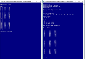
A good way to understand what k-means++ clustering is and to see where this article is headed is to examine the screenshot of a demo program in Figure 1. The goal of the demo is to cluster a simple dataset of 20 items. Each item represents the height (in inches) and weight (in pounds) of a person. The data has been normalized by dividing all height values by 100 and all weight values by 1000. The k-means algorithm uses the Euclidean distance between data items. This means that data items must be purely numeric and the values should be normalized so that variables with large magnitudes (such as an annual income of 58,000.00) don't dominate variables with small magnitudes (such as an age of 32.0).
The demo data is artificial and is constructed so that there are three clear clusters. However, even for this simple problem with N = 20 and dim = 2, the way the data items are related is not clear at all.
The demo program begins by preparing the clustering function. The number of clusters is set to k = 3. Data clustering is an exploratory process and in almost all cases a good number for k must be determined by trial and error. In the second part of this article, I describe two techniques, the Elbow technique and the Knee technique, that can help determine a good value for k.
The demo code has been designed so that you can easily experiment with other k-means initialization techniques. The initialization technique is set to "plusplus." After the initialization phase of k-means, the algorithm is iterative so the demo sets a maximum number of iterations to 100. In most cases k-means converges to a result clustering quickly (but not necessarily the optimal result), so maxIter is an upper limit on the number of iterations, not the actual number of iterations performed.
The k-means++ initialization technique has a random component so a seed value for the random number generator is set to 0. This seed value is arbitrary. In general, the effectiveness of k-means++ initialization is not heavily influenced by the choice of seed value used.
On a single clustering attempt, k-means with any initialization technique could return a poor clustering. The standard approach is to try k-means several times, keeping track of the best clustering result found. The demo sets a variable named trials to 10. Unlike the maxIter variable, the trials variable is a fixed number of iterations, not an upper iteration limit.
The demo then clusters the data 10 times and displays an array that holds the best clustering found: (1, 2, 0, 0, 2, 1, . . 0). The cell value is a cluster ID, and the cell indexes indicate which data item. So, data item [0] is in cluster 1, data [1] is in cluster 2, data [2] is in cluster 0, and so on to data [19] in cluster 0.
The demo displays the number of data items in each cluster: (7, 8, 5) which means 7 data items are in cluster 0, 8 items in cluster 1, and 5 items in cluster 2.
The k-means algorithm computes the mean of the data items in each cluster: (0.6014, 0.1171), (0.6750, 0.2212), (0.7480, 0.1700). The cluster means are sometimes called cluster centers or cluster centroids.
The demo displays the total within-cluster sum of squares (WCSS) value: 0.0072. The total WCSS is a measure of how good a particular clustering of data is. Smaller values are better. There is a WCSS for each cluster, computed as the sum of the squared differences between data items in a cluster and their cluster mean. The total WCSS is the sum of the WCSS values for each cluster. The k-means algorithm minimizes the total WCSS.
The demo concludes by displaying the data by cluster. The clustered data make it clear that there are three types of people: short people with light weights in cluster 0, medium-height heavy people in cluster 1, and tall people with medium weights in cluster 2. Cluster IDs are not meaningful and on a different run, the same data items would be clustered together but the three cluster IDs could be rearranged.
 [Click on image for larger view.] Figure 1: K-Means++ Clustering in Action
This article assumes you have intermediate or better skill with C# but doesn’t assume you know anything about k-means clustering with k-means++ initialization. The code for demo program is too long to present in its entirety in this article but the complete code is available in the associated file download. All normal error checking has been removed to keep the main ideas as clear as possible
Understanding K-Means++ Initialization
In pseudo-code, the generic k-means clustering algorithm is:
initialize the k means
use means to initialize clustering
loop at most maxIter times
use new clustering to update means
  use new means to update clustering
  exit loop if no change to clustering or
    clustering would create an empty cluster
end-loop
return clustering
The first two steps, initializing the means and then the clustering, are what distinguish the different types of k-means clustering. Forgy initialization selects k data items at random and uses the values of the selected items for the k means. Random initialization assigns every data item to one of the clusters and then computes the k means from the initial clustering.
After the means and clustering have been initialized, the k-means algorithm is deterministic. Therefore, how well k-means works depends entirely on the initialization. As it turns out, the more different the initial k means are, the more likely you are to get a good clustering. With Forgy initialization and random initialization, you might get good initial means that are different from each other but you could get bad initial means too.
The k-means++ initialization technique finds initial means that are very different from each other. In pseudo-code:
pick one data item at random
use those values as first mean
loop for remaining k-1 means
  compute distance of each data item to
    all existing means
  pick an item that is far from its closest mean
  use that far item's values as next mean
end-loop
The k-means++ initialization algorithm is quite subtle. The part of the algorithm "pick an item that is far from its closest mean" is the key. Suppose you have a problem with k = 4 and suppose at some point you have the first two of the four means determined. To determine the values for the third mean, you compute the distances from each data item to its closest mean, which could be either of the first two means. Then you randomly select one of the data items with probability equal to the squared distance divided by the sum of all the squared distances.
For example, suppose there are just four data items. And suppose the first two of the data items are closest to mean [0] and the third and fourth items are closest to mean [1]. And the distances of the four items to their closest mean are 2.0, 5.0, 3.0, 4.0. The squared distances are 4.0, 25.0, 9.0, 16.0. The sum of the squared distances is 54.0. The k-means++ algorithm picks one of the four data items for the third mean using probabilities 4/54 = 0.07, 25/54 = 0.46, 9/54 = 0.17, 16/54 = 0.30. Any of the four data items could be selected for use as the third mean, but the one that's farthest from its closest mean is the one most likely to be picked.
You might be wondering why k-means++ uses squared distances rather than plain distances. One reason is that using squared distances gives more weight to larger distances away from means (which is good). For example, if you used the plain distances of 2, 5, 3, 4, the probabilities of each being selected would be 2/14 = 0.14, 5/14 = 0.36, 3/14 = 0.21, 4/14 = 0.29. The second item still has the largest probability of being selected (p = 0.36) but not as likely as it is when using squared distances (p = 0.46).
To summarize, the behavior of k-means clustering depends upon how the means are initialized. Means that are different from each other are better. The k-means++ initialization algorithms picks data items based on probabilities calculated from the squared distances of data items to their closest mean.
Roulette Wheel Selection
There are several ways to pick one value from a set of values in a way that is proportional to the sum of the values. The demo program uses a mini-algorithm called roulette wheel selection. Suppose you have an array of five values.
 20   50   30   60   40
[0]  [1]  [2]  [3]  [4]
The sum of the five values is 200. You want the probabilities of selection for each item to be the value divided by the sum of the five values:
  0.10   0.25   0.15   0.30   0.20
  [0]    [1]    [2]    [3]    [4]
So, item [3] has the largest probability of being selected but any of the five values could be selected. For roulette wheel selection, you compute an array of cumulative probabilities:
  0.00   0.10   0.35   0.50   0.80   1.00
  [0]    [1]    [2]    [3]    [4]    [5]
Notice the cumulative probabilities array has one more cell than the number of items to select from. The first and last cells of the cumulative probabilities array will always be 0.0 and 1.0 respectively. Also, notice that that difference in consecutive values of the cumulative probabilities array correspond to the probabilities of each item being selected.
To select one item, you generate a random p value between 0.0 and 1.0. Suppose p = 0.77. You walk through the cumulative array starting at index [0], looking at the value in the next cell. You stop and return the current index value when the next-cell value exceeds the p value.
At index [0] the next cell holds 0.10 which doesn't exceed p = 0.77 so you advance to index [1]. The next cell holds 0.35 which doesn't exceed p so you advance to index [2]. The next cell holds 0.50 which doesn't exceed p so you advance to index [3]. The next cell holds 0.80 which does exceed p = 0.77 so you stop and return [3] as the selected index.
When implementing roulette wheel selection, you don't need to pre-compute all the cumulative probabilities. Instead you can compute the cumulative probabilities on the fly which avoids a few unneeded computations. The demo program uses the on-the-fly approach. The code implementation is presented in Listing 1.
Listing 1. Roulette Wheel Proportional Selection
static int ProporSelect(double[] vals, Random rnd)
{
  // roulette wheel selection
  // on the fly technique
  // vals[] can't be all 0.0s
  int n = vals.Length;

  double sum = 0.0;
  for (int i = 0; i < n; ++i)
    sum += vals[i];

  double cumP = 0.0;  // cumulative prob
  double p = rnd.NextDouble();

  for (int i = 0; i < n; ++i) {
    cumP += (vals[i] / sum);
    if (cumP > p) return i;
  }
  return n - 1;  // last index
}
The demo implementation doesn't perform any error checking, such as verifying that the vals array parameter doesn't have all 0.0 contents which would give a divide by zero error. Adding only the error checking you need for a particular programming scenario is both a strength and weakness of implementing machine learning from scratch.
The Demo Program
To create the demo program, I launched Visual Studio 2019. I used the Community (free) edition but any relatively recent version of Visual Studio will work fine. From the main Visual Studio start window I selected the "Create a new project" option. Next, I selected C# from the Language dropdown control and Console from the Project Type dropdown, and then picked the "Console App (.NET Core)" item.
The code presented in this article will run as a .NET Core console application or as a .NET Framework application. Many of the newer Microsoft technologies, such as the ML.NET code library, specifically target .NET Core so it makes sense to develop most new C# machine learning code in that environment.
I entered "ClusteringKM" as the Project Name, specified C:\VSM on my local machine as the Location (you can use any convenient directory), and checked the "Place solution and project in the same directory" box.
After the template code loaded into Visual Studio, at the top of the editor window I removed all using statements to unneeded namespaces, leaving just the reference to the top-level System namespace. In a non-demo scenario you'll likely need the System.IO namespace to read data into memory from a text file. The demo needs no other assemblies and uses no external code libraries.
In the Solution Explorer window, I renamed file Program.cs to the more descriptive ClusteringKMProgram.cs and then in the editor window I renamed class Program to class ClusteringKMProgram to match the file name. The structure of the demo program, with a few minor edits to save space, is shown in Listing 2.
Listing 2. K-Means++ Demo Program Structure
using System;
// using System.IO;
namespace ClusteringKM
{
  class ClusteringKMProgram
  {
    static void Main(string[] args)
    {
      Console.WriteLine("Begin k-means++ demo ");

      double[][] data = new double[20][];
      data[0] = new double[] { 0.65, 0.220 };
      data[1] = new double[] { 0.73, 0.160 };
      . . .
      data[19] = new double[] { 0.61, 0.130 };

      Console.WriteLine("Data: ");
      ShowMatrix(data, new int[] { 2, 3 },
        new int[] { 5, 8 }, true);

      Console.WriteLine("Press Enter ");
      Console.ReadLine();  // pause

      int k = 3;  // number clusters
      string initMethod = "plusplus";
      int maxIter = 100;
      int seed = 0;

      Console.WriteLine("Setting k = " + k);
      Console.WriteLine("Setting initMethod = " +
        initMethod);
      Console.WriteLine("Setting maxIter = " +
        maxIter);
      Console.WriteLine("Setting seed = " + seed);
      KMeans km = new KMeans(k, data, initMethod,
        maxIter, seed);

      int trials = 10;  // attempts to find best
      Console.WriteLine("Clustering w/ trials = " +
        trials);
      km.Cluster(trials);
      Console.WriteLine("Done");

      Console.WriteLine("Best clustering found: ");
      ShowVector(km.clustering, 3);

      Console.WriteLine("Cluster counts: ");
      ShowVector(km.counts, 4);

      Console.WriteLine("The cluster means: ");
      ShowMatrix(km.means, new int[] { 4, 4 },
        new int[] { 8, 8 }, true);

      Console.WriteLine("Within-cluster SS = " +
        km.wcss.ToString("F4"));

      Console.WriteLine("Clustered data: ");
      ShowClustered(data, k, km.clustering,
        new int[] { 2, 3 },
        new int[] { 8, 10 }, true);

      Console.WriteLine("End demo");
      Console.ReadLine();
    } // Main

    static void ShowVector(int[] vec, int wid) { . . }

    static void ShowMatrix(double[][] m, int[] dec,
      int[] wid, bool indices) { . . }

    static void ShowClustered(double[][] data, int K,
      int[] clustering, int[] decs, int[] wids,
      bool indices) { . . }
  } // Program

  public class KMeans
  {
   . . .
  }

} // ns
All of the program control logic is contained in the Main() method. All of the clustering logic is contained in a KMeans class. The demo begins by setting up the source data:
double[][] data = new double[20][];
data[0] = new double[] { 0.65, 0.220 };
data[1] = new double[] { 0.73, 0.160 };
. . .
data[19] = new double[] { 0.61, 0.130 };
The demo data is hard-coded and stored into an array-of-arrays style matrix. In a non-demo scenario you'd likely read your data into memory from a text file, using a helper function along the lines of:
string fn = "..\\..\\..\\Data\\my_data.txt";
double[][] data = MatLoad(fn, 20,
  new int[] { 0, 1, 4 }, '\t');
This means, "read 20 lines, columns 0, 1 and 4 of the data file (skipping lines that begin with "//") from file my_data.txt where values are separated by tab characters." The demo program in the file download that accompanies this article has an implementation of the MatLoad() function.
After setting up the training data, the demo program displays the data using these statements:
Console.WriteLine("Data: ");
ShowMatrix(data, new int[] { 2, 3 },
  new int[] { 5, 8 }, true);
Console.WriteLine("Press Enter to continue ");
Console.ReadLine();  // pause
The ShowMatrix() helper function pretty-prints an array-of-arrays. The function accepts the number of decimals and the width to display for the values in each column (with blank space padding). The function has a Boolean parameter that controls whether to display row indices or not.
The clustering is prepared by setting up values for the KMeans constructor and instantiating a KMeans object:
int k = 3;
string initMethod = "plusplus";
int maxIter = 100;
int seed = 0;
KMeans km = new KMeans(k, data, initMethod,
  maxIter, seed);
The demo program only supports the k-means++ initialization but has been designed to easily support other initialization schemes. The data is clustered like so:
int trials = 10;  // attempts to find best
Console.WriteLine("Clustering w/ trials = " +
  trials);
km.Cluster(trials);
Console.WriteLine("Done");
The Cluster() method will iterate 10 times. On each iteration, the k-means++ initialization technique is used. The method keeps track of the best clustering found. The number of trials to use is problem-dependent and must be determined by trial and error.
The demo displays clustering results, starting with the clustering itself:
Console.WriteLine("Best clustering found: ");
ShowVector(km.clustering, 3);

Console.WriteLine("Cluster counts: ");
ShowVector(km.counts, 4);
Helper function ShowVector() accepts a width argument. Because the demo data has only 20 items, it's feasible to display the entire clustering array. Examining the number of data items assigned to each cluster can reveal unusual clusters that you might want to take a closer look at. The clustering method is designed to prevent any cluster count of 0, so if you see a zero count you should investigate.
The demo displays the cluster means using a ShowMatrix() helper function that accepts per-column decimals and widths arguments:
Console.WriteLine("The cluster means: ");
ShowMatrix(km.means, new int[] { 4, 4 },
  new int[] { 8, 8 }, true);
Examining the cluster means can give you insights about how close the clusters are. A cluster mean can be thought of as a representative value of a cluster of data. There are several machine learning algorithms that perform k-means clustering in an initialization phase, and then use the cluster means.
Next the demo displays the total within-cluster sum of squares:
Console.WriteLine("Within-cluster SS = " +
  km.wcss.ToString("F4"));
The total WCSS can be used to compare the quality of different clusterings on a particular dataset, where smaller values are better. The scale of the total WCSS is data-dependent so you can't compare total WCSS values for different datasets. In some cases you might want to display the individual WCSS values for each cluster.
The demo concludes by displaying the source data by cluster assignment:
Console.WriteLine("Clustered data: ");
ShowClustered(data, k, km.clustering,
  new int[] { 2, 3 },
  new int[] { 8, 10 }, true);
The ShowClustered() helper function accepts arguments for the number of decimals for each column, and the widths to use for each column.
The Elbow and Knee Techniques
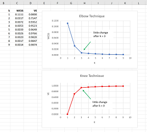
The Elbow and Knee techniques can be used to determine a good value for the number of clusters for a dataset. The idea of the Elbow technique is to cluster a dataset using different values of k and then graphing the values of the total WCSS. The top image in Figure 2 shows the graph of the Elbow technique for the demo dataset.
 [Click on image for larger view.] Figure 2: The Elbow and Knee Techniques
When k = 1 the total WCSS is the largest possible value for a dataset. It is the total variability in the data. The larger the value of k, the smaller the value of the total WCSS will be. In the extreme, if k equals the number of items in a dataset, the total WCSS will be 0. In datasets where there is a natural clustering, the graph of WCSS will decrease and at some point the change in WCSS will relatively small. This means that using more clusters doesn't add much information.
The code that generated the WCSS values for the demo data is:
for (int k = 1; k <= 9; ++k) {
  KMeans km = new KMeans(k, data,
    "plusplus", 100, seed: k);
  km.Cluster(10);
  Console.WriteLine(k + " " +
    km.wcss.ToString("F4"));
}
The Knee technique is really the same as the Elbow technique. One minor disadvantage of the Elbow technique is that the magnitude of WCSS values depend on the data being clustered, and so you can't easily compare different datasets. The Knee technique converts raw WCSS values into percentages of variability explained (VE). For example, for the demo data, the total variability is when k = 1 and is 0.1111. The percent VE for a given value of k is (0.1111 - WCSS(k)) / 0.1111. For any dataset the percent VE will range from 0 to 1 and you can think of VE as normalized WCSS.
Some resources state that the Knee technique uses the percentage of statistical variance explained, instead of the percentage of variability explained. The percentage of variability explained is the same as the percentage of statistical variance explained. Statistical variance is variability divided by the degrees of freedom, df. For clustering problems df = n-1 where n is the number of data items. For clustering problems, df will be constant for a particular dataset and when computing percentage of statistical variance, the df terms cancel out.
The Elbow and Knee techniques are subjective ways to determine a good k value for data clustering. In most non-demo scenarios the graphs won't be as easy to interpret as those in Figure 2.
Wrapping Up
The k-means clustering algorithm with k-means++ initialization is relatively simple, easy to implement, and effective. One disadvantage of k-means clustering is that it only works with strictly numeric data. Attempting to use k-means with non-numeric data by encoding doesn't work well. For example, suppose a column of source data is one of three colors, red, blue, green. If you encode red = 1, blue = 2, green = 3 then the distance between red and blue is less then the distance between red and green, which doesn't make sense. Or if you encode red = (1, 0, 0), blue = (0, 1, 0), green = (0, 0, 1) you don't help yourself much because the Euclidean distance between any two different colors is sqrt(2.0) which doesn't add any useful information.
Clustering non-numeric, or mixed numeric and non-numeric data is surprisingly difficult. For strictly non-numeric data one approach is to use techniques based on a metric called category utility. For mixed numeric and non-numeric data one approach is to use a metric called Gower distance. Another approach for clustering mixed numeric and non-numeric data is to encode the data using a neural network autoencoder and then use k-means with k-means++ initialization.