The Data Science Lab
Multi-Class Classification Using PyTorch: Training
Dr. James McCaffrey of Microsoft Research continues his four-part series on multi-class classification, designed to predict a value that can be one of three or more possible discrete values, by explaining neural network training.
The goal of a multi-class classification problem is to predict a value that can be one of three or more possible discrete values, such as "poor," "average" or "good" for a loan applicant's credit rating. This article is the third in a series of four articles that present a complete end-to-end production-quality example of multi-class classification using a PyTorch neural network. The running example problem is to predict a college student's major ("finance," "geology" or "history") from their sex, number of units completed, home state and score on an admission test.
The process of creating a PyTorch neural network multi-class classifier consists of six steps:
- Prepare the training and test data
- Implement a Dataset object to serve up the data
- Design and implement a neural network
- Write code to train the network
- Write code to evaluate the model (the trained network)
- Write code to save and use the model to make predictions for new, previously unseen data
Each of the six steps is complicated. And the six steps are tightly coupled which adds to the difficulty. This article covers the fourth step -- training a neural network for multi-class classification.
A good way to see where this series of articles is headed is to take a look at the screenshot of the demo program in Figure 1. The demo begins by creating Dataset and DataLoader objects which have been designed to work with the student data. Next, the demo creates a 6-(10-10)-3 deep neural network. The demo prepares training by setting up a loss function (cross entropy), a training optimizer function (stochastic gradient descent) and parameters for training (learning rate and max epochs).
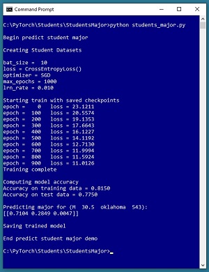 [Click on image for larger view.] Figure 1: Predicting Student Major Multi-Class Classification in Action
The demo trains the neural network for 1,000 epochs in batches of 10 items. An epoch is one complete pass through the training data. The training data has 200 items, therefore, one training epoch consists of processing 20 batches of 10 training items.
During training, the demo computes and displays a measure of the current error (also called loss) every 100 epochs. Because error slowly decreases, it appears that training is succeeding. This is good because training failure is usually the norm rather than the exception. Behind the scenes, the demo program saves checkpoint information after every 100 epochs so that if the training machine crashes, training can be resumed without having to start from the beginning.
After training the network, the demo program computes the classification accuracy of the model on the training data (163 out of 200 correct = 81.50 percent) and on the test data (31 out of 40 correct = 77.50 percent). Because the two accuracy values are similar, it's likely that model overfitting has not occurred.
Next, the demo uses the trained model to make a prediction. The raw input is (sex = "M", units = 30.5, state = "oklahoma", score = 543). The raw input is normalized and encoded as (sex = -1, units = 0.305, state = 0, 0, 1, score = 0.5430). The computed output vector is [0.7104, 0.2849, 0.0047]. These values represent the pseudo-probabilities of student majors "finance," "geology," and "history" respectively. Because the probability associated with "finance" is the largest, the predicted major is "finance."
The demo concludes by saving the trained model using the state dictionary approach. This is the most common of three standard techniques.
This article assumes you have an intermediate or better familiarity with a C-family programming language, preferably Python, but doesn't assume you know very much about PyTorch. The complete source code for the demo program, and the two data files used, are available in the download that accompanies this article. All normal error checking code has been omitted to keep the main ideas as clear as possible.
To run the demo program, you must have Python and PyTorch installed on your machine. The demo programs were developed on Windows 10 using the Anaconda 2020.02 64-bit distribution (which contains Python 3.7.6) and PyTorch version 1.7.0 for CPU installed via pip. Installation is not trivial. You can find detailed step-by-step installation instructions for this configuration in my blog post.
The Student Data
The raw Student data is synthetic and was generated programmatically. There are a total of 240 data items, divided into a 200-item training dataset and a 40-item test dataset. The raw data looks like:
M  39.5  oklahoma  512  geology
F  27.5  nebraska  286  history
M  22.0  maryland  335  finance
. . .
M  59.5  oklahoma  694  history
Each line of tab-delimited data represents a hypothetical student at a hypothetical college. The fields are sex, units-completed, home state, admission test score and major. The first four values on each line are the predictors (often called features in machine learning terminology) and the fifth value is the dependent value to predict (often called the class or the label). For simplicity, there are just three different home states and three different majors.
The raw data was normalized by dividing all units-completed values by 100 and all test scores by 1000. Sex was encoded as "M" = -1, "F" = +1. The home states were one-hot encoded as "maryland" = (1, 0, 0), "nebraska" = (0, 1, 0), "oklahoma" = (0, 0, 1). The majors were ordinal encoded as "finance" = 0, "geology" = 1, "history" = 2. Ordinal encoding for the dependent variable, rather than one-hot encoding, is required for the neural network design presented in the article. The normalized and encoded data looks like:
-1  0.395  0 0 1  0.5120  1
 1  0.275  0 1 0  0.2860  2
-1  0.220  1 0 0  0.3350  0
. . .
-1  0.595  0 0 1  0.6940  2
After the structure of the training and test files was established, I coded a PyTorch Dataset class to read data into memory and serve the data up in batches using a PyTorch DataLoader object. A Dataset class definition for the normalized encoded Student data is shown in Listing 1.
Listing 1: A Dataset Class for the Student Data
class StudentDataset(T.utils.data.Dataset):
  def __init__(self, src_file, n_rows=None):
    all_xy = np.loadtxt(src_file, max_rows=n_rows,
      usecols=[0,1,2,3,4,5,6], delimiter="\t",
      skiprows=0, comments="#", dtype=np.float32)

    n = len(all_xy)
    tmp_x = all_xy[0:n,0:6]  # all rows, cols [0,5]
    tmp_y = all_xy[0:n,6]    # 1-D required

    self.x_data = \
      T.tensor(tmp_x, dtype=T.float32).to(device)
    self.y_data = \
      T.tensor(tmp_y, dtype=T.int64).to(device)

  def __len__(self):
    return len(self.x_data)

  def __getitem__(self, idx):
    preds = self.x_data[idx]
    trgts = self.y_data[idx]
    sample = {
      'predictors' : preds,
      'targets' : trgts
    }
    return sample
Preparing data and defining a PyTorch Dataset is not trivial. You can find the article that explains how to create Dataset objects and use them with DataLoader objects in The Data Science Lab.
The Neural Network Architecture
In the previous article in this series, I described how to design and implement a neural network for multi-class classification for the Student data. One possible definition is presented in Listing 2. The code defines a 6-(10-10)-3 neural network with tanh() activation on the hidden nodes.
Listing 2: A Neural Network for the Student Data
class Net(T.nn.Module):
  def __init__(self):
    super(Net, self).__init__()
    self.hid1 = T.nn.Linear(6, 10)  # 6-(10-10)-3
    self.hid2 = T.nn.Linear(10, 10)
    self.oupt = T.nn.Linear(10, 3)

    T.nn.init.xavier_uniform_(self.hid1.weight)
    T.nn.init.zeros_(self.hid1.bias)
    T.nn.init.xavier_uniform_(self.hid2.weight)
    T.nn.init.zeros_(self.hid2.bias)
    T.nn.init.xavier_uniform_(self.oupt.weight)
    T.nn.init.zeros_(self.oupt.bias)

  def forward(self, x):
    z = T.tanh(self.hid1(x))
    z = T.tanh(self.hid2(z))
    z = self.oupt(z)  # CrossEntropyLoss()
    return z
If you are new to PyTorch, the number of design decisions for a neural network can seem daunting. But with every program you write, you learn which design decisions are important and which don't affect the final prediction model very much, and the pieces of the puzzle eventually fall into place.
The Overall Program Structure
The overall structure of the PyTorch multi-class classification program, with a few minor edits to save space, is shown in Listing 3. I indent my Python programs using two spaces rather than the more common four spaces.
Listing 3: The Structure of the Demo Program
# students_major.py
# PyTorch 1.7.0-CPU Anaconda3-2020.02
# Python 3.7.6 Windows 10

import numpy as np
import time
import torch as T
device = T.device("cpu")

class StudentDataset(T.utils.data.Dataset):
  def __init__(self, src_file, n_rows=None): . . .
  def __len__(self): . . .
  def __getitem__(self, idx): . . .

# ----------------------------------------------------

def accuracy(model, ds): . . .

# ----------------------------------------------------

class Net(T.nn.Module):
  def __init__(self): . . .
  def forward(self, x): . . .

# ----------------------------------------------------

def main():
  # 0. get started
  print("Begin predict student major ")
  np.random.seed(1)
  T.manual_seed(1)

  # 1. create Dataset and DataLoader objects
  # 2. create neural network
  # 3. train network
  # 4. evaluate accuracy of model
  # 5. make a prediction
  # 6. save model

  print("End predict student major demo ")

if __name__== "__main__":
  main()
It's important to document the versions of Python and PyTorch being used because both systems are under continuous development. Dealing with versioning incompatibilities is a significant headache when working with PyTorch and is something you should not underestimate.
I like to use "T" as the top-level alias for the torch package. Most of my colleagues don't use a top-level alias and spell out "torch" dozens of times per program. Also, I use the full form of sub-packages rather than supplying aliases such as "import torch.nn.functional as functional". In my opinion, using the full form is easier to understand and less error-prone than using many aliases.
The demo program defines a program-scope CPU device object. I usually develop my PyTorch programs on a desktop CPU machine. After I get that version working, converting to a CUDA GPU system only requires changing the global device object to T.device("cuda") plus a minor amount of debugging.
The demo program defines just one helper method, accuracy(). All of the rest of the program control logic is contained in a single main() function. It is possible to define other helper functions such as train_net(), evaluate_model() and save_model(), but in my opinion this modularization approach unexpectedly makes the program more difficult to understand rather than easier to understand.
Training the Neural Network
The details of training a neural network with PyTorch are complicated but the code is relatively simple. In very high-level pseudo-code, the process to train a neural network looks like:
      loop max_epochs times
        loop until all batches processed
          read a batch of training data (inputs, targets)
          compute outputs using the inputs
          compute error between outputs and targets
          use error to update weights and biases
        end-loop (all batches)
      end-loop (all epochs)
The difficult part of training is the "use error to update weights and biases" step. PyTorch does most, but not all, of the hard work for you. It's not easy to understand neural network training without seeing a working program. The program shown in Listing 4 demonstrates how to train a network for multi-class classification. The screenshot in Figure 2 shows the output from the test program.
Listing 4: Testing Neural Network Training Code
# test_training.py

import numpy as np
import time
import torch as T
device = T.device("cpu")

class StudentDataset(T.utils.data.Dataset):
  # see Listing 1

class Net(T.nn.Module):
  # see Listing 2

print("Begin test of training ")

T.manual_seed(1)
np.random.seed(1)
train_file = ".\\Data\\students_train.txt"
train_ds = StudentDataset(train_file, n_rows=200)

bat_size = 10
train_ldr = T.utils.data.DataLoader(train_ds,
  batch_size=bat_size, shuffle=True)

net = Net().to(device)
net.train()  # set mode

lrn_rate = 0.01
loss_func = T.nn.CrossEntropyLoss()
optimizer = T.optim.SGD(net.parameters(),
  lr=lrn_rate)

for epoch in range(0, 100):
  # T.manual_seed(1 + epoch)  # recovery reproducibility
  epoch_loss = 0.0  # sum avg loss per item

  for (batch_idx, batch) in enumerate(train_ldr):
    X = batch['predictors']  # inputs
    Y = batch['targets']     # shape [10,3] (!)

    optimizer.zero_grad()
    oupt = net(X)            # shape [10] (!)

    loss_val = loss_func(oupt, Y)  # avg loss in batch
    epoch_loss += loss_val.item()  # a sum of averages
    loss_val.backward()
    optimizer.step()

  if epoch % 10 == 0:
    print("epoch = %4d   loss = %0.4f" % \
     (epoch, epoch_loss))
    # TODO: save checkpoint

print("Done ")
The training demo program begins execution with:
T.manual_seed(1)
np.random.seed(1)
train_file = ".\\Data\\students_train.txt"
train_ds = StudentDataset(train_file, n_rows=200)
The global PyTorch and NumPy random number generator seeds are set so that results will be reproducible. Unfortunately, due to multiple threads of execution, in some cases your results will not be reproducible even if you set the seed values.
The demo assumes that the training data is located in a subdirectory named Data. The StudentDataset object reads all 200 training data items into memory. If your training data size is very large you can read just part of the data into memory using the n_rows parameter.
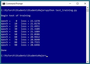 [Click on image for larger view.] Figure 2: Testing the Training Code
The demo program prepares training with these statements:
bat_size = 10
train_ldr = T.utils.data.DataLoader(train_ds,
  batch_size=bat_size, shuffle=True)
net = Net().to(device)
net.train()  # set mode
The training data loader is configured to read batches of 10 items at a time. In theory, the batch size doesn't matter, but in practice the batch size greatly affects how quickly training works. When you have a choice, it makes sense to use a batch size that divides the dataset size evenly so that all batches have the same size. Because the demo test Student data has 200 rows, there will be 20 batches of 10 items each and no leftover items. It is very important to set shuffle=True when training because the default value is False which will usually result in failed training.
After the neural network is created, it is set into training mode using the statement net.train(). If your neural network has a dropout layer or a batch normalization layer, you must set the network to train() mode during training and to eval() mode when using the network at any other time, such as making a prediction or computing model classification accuracy. The default state is train() mode so setting the mode isn't necessary for the demo network for two reasons: it's already in train() mode, and it doesn't use dropout or batch normalization. However, in my opinion it's good practice to always explicitly set the network mode. The train() mode method works by reference so you can write just net.train() instead of net = net.train(). Note that the statement net.train() looks like it's an instruction to train a net object, but that is not what's happening.
The demo continues training preparation with these three statements:
lrn_rate = 0.01
loss_func = T.nn.CrossEntropyLoss()
optimizer = T.optim.SGD(net.parameters(),
  lr=lrn_rate)
For multi-class classification, the two main loss (error) functions are cross entropy error and mean squared error. In the early days of neural networks, mean squared error was more common but now cross entropy is far more common.
The CrossEntropyLoss() object is actually a wrapper around applying log_softmax() activation on the output nodes, combined with using the NLLLoss() method ("negative log likelihood loss") during training. Therefore, when using CrossEntropyLoss() you do not apply explicit activation on the output nodes in the forward() method. One of the most common mistakes when using PyTorch for multi-class classification is to apply softmax() or log_softmax() to the output nodes in the forward() method of the network class definition, and then use the CrossEntropyLoss() function. This mistake will not generate an error or warning message, but it will slow training down, or in some cases cause training to fail.
The demo program uses the simplest possible training optimization technique which is stochastic gradient descent (SGD). Understanding all the details of PyTorch optimizers is extremely difficult. PyTorch 1.7 supports 11 different techniques. Each technique's method has several parameters which are very complex and which often have a dramatic effect on training performance. See the list in Figure 3.
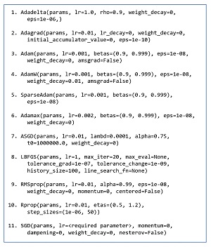 [Click on image for larger view.] Figure 3: PyTorch Optimizers
Fortunately, almost all of the PyTorch optimizer parameters have reasonable default values. As a general rule of thumb, for multi-class classification problems I start by trying SGD with default parameter values. Then if SGD fails after a few hours of experimentation with its parameters, I try the Adam algorithm (Adam is not an acronym but its name derives from "adaptive moment estimation"). In theory, any one of the PyTorch optimizers will work -- there is no magic algorithm. Loosely expressed, the key difference between SGD and Adam is that SGD uses a single fixed learning rate for all weights and biases, but Adam uses a dedicated, adaptive learning rate for each weight and bias.
A learning rate controls how much a network weight or bias changes on each update during training. For SGD, a small learning rate will slowly but surely improve weights and biases, but the changes might be so slow that training takes too long. A large learning rate trains a neural network faster but at the risk of jumping past a good weight or bias value and missing it.
The key takeaway is that if you're new to PyTorch you could easily spend weeks exploring the nuances of different training optimizers and never get any programs written. Optimizers are important but it's better to learn about different optimizers by experimenting with them slowly over time, with different problems, than it is to try and master all their details before writing any code.
After training has been prepared, the demo program starts the training:
for epoch in range(0, 100):
  # T.manual_seed(1 + epoch)  # recovery reproducibility
  epoch_loss = 0.0            # sum avg loss per item
  for (batch_idx, batch) in enumerate(train_ldr):
    X = batch['predictors']   # inputs
    Y = batch['targets']      # shape [10,3]
    optimizer.zero_grad()
    oupt = net(X)             # shape [10]
. . .
Setting the manual seed inside the main training loop is necessary if you periodically save the model's weights and biases as checkpoints, so that if the training machine crashes during training, you can recover. Because the demo program doesn't save checkpoints, it's not necessary to set the seed, which is why that statement is commented out.
For each batch of 10 items, the 10 sets of inputs are extracted as X and the 10 target values are extracted as Y. The inputs are fed to the network and the results are captured as oupt. The zero_grad() method resets the gradients of all weights and biases so that new gradients can be computed and used to update the weights and biases.
The demo continues with:
  loss_val = loss_func(oupt, Y)  # avg loss in batch
  epoch_loss += loss_val.item()  # a sum of averages
  loss_val.backward()            # compute gradients
  optimizer.step()               # update weights
It's important to monitor the cross entropy error/loss during training so that you can tell if training is working or not. There are three main ways to monitor loss. An epoch_loss value is computed for each batch of input values. This batch loss value is the average of the loss values for each item in the batch. For example, if a batch has four items and the cross entropy loss values for each of the four items are (8.00, 2.00, 5.00, 3.00) then the computed batch loss is 18.00 / 4 = 4.50. The simplest approach is to just display the loss for either the first batch or the last batch for each training epoch. It's usually not feasible to print the loss value for every batch because there are just too many batches processed in almost all realistic scenarios.
A second approach for monitoring loss during training is to accumulate each batch loss value, and then after all the batches in one epoch have been processed in one epoch, you can display the sum of the batch losses. For example, if one epoch consists of 3 batches of data and the batch average loss values are (3.50, 6.10, 2.30) then the sum of the batch losses is 3.50 + 6.10 + 2.30 = 11.90. This approach for monitoring loss is the one used by the demo program.
A third approach for monitoring loss is to compute an average loss per item for all training items. This is a bit tricky. First you would "un-average" the average loss value returned by the loss_func() method, by multiplying by the number of items in the batch, and then you'd accumulate the individual loss values. After all batches have been processed, you can compute an average loss per item over the entire dataset by dividing by the total number of training items. The code would look like this:
for epoch in range(0, 100):
  sum_epoch_loss = 0.0

  for (batch_idx, batch) in enumerate(train_ldr):
    . . .
    loss_val = loss_func(oupt, Y)  # avg loss in batch
    sum_vals = loss_val.item() * len(X)  # "un-average"
    sum_epoch_loss += sum_vals           # accumulate
    . . .

  if epoch % 10 == 0:
    avg_loss = sum_epoch_loss / len(train_ds)  # average
    print(avg_loss)
None of the three approaches for monitoring loss during training give values that are easy to interpret. The important thing is to watch the values to see if they are decreasing. It is possible for training loss to values to bounce around a bit, where a loss value might increase briefly, especially if your batch size is small. Because there are many ways to monitor and display cross entropy loss for multi-class classification, loss values usually can't be compared for different systems unless you know the systems are computing and displaying loss in the exact same way.
The item() method is used when you have a tensor that has a single numeric value. The item() method extracts the single value from the associated tensor and returns it as a regular scalar value. Somewhat unfortunately (in my opinion), PyTorch 1.7 allows you to skip the call to item() so you can write the shorter epoch_loss += loss_val instead. Because epoch_loss is a non-tensor scalar, the interpreter will figure out that you must want to extract the value in the loss_val tensor. You can think of this mechanism as similar to implicit type conversion. However, the shortcut form with item() is misleading in my opinion and so I use item() in most situations, even when it's not technically necessary.
The loss_val is a tensor that is the last value in the behind-the-scenes computational graph that represents the neural network being trained. The loss_val.backward() method uses the back-propagation algorithm to compute all the gradients associated with the weights and biases that a part of the network containing loss_val. Put another way, loss_val.backward() computes the gradients of the output node weights and bias, and then the hid2 layer gradients, and then the hid1 layer gradients.
The optimizer.step() statement uses the newly computed gradients to update all the weights and biases in the neural network so that computed output values will get closer to the target values. When you instantiate an optimizer object for a neural network, you must pass in the network parameters object and so the optimizer object effectively has full access to the network and can modify it.
The demo program concludes training with these statements:
. . .
    optimizer.step()

  if epoch % 10 == 0:
    print("epoch = %4d   loss = %0.4f" % \
      (epoch, epoch_loss))
    # TODO: save checkpoint

print("Done ")
After all batches have been processed, a training epoch has been completed and program execution exits the innermost for-loop. Although it's possible to display the accumulated loss value for every epoch, in most cases that's too much information and so the demo just displays the accumulated loss once every 10 epochs. In many problem scenarios you might want to store all accumulated epoch loss values in memory, and then save them all to a text file after training completes. This allows you to analyze training without slowing it down.
Because training a neural network can take hours, days, or even longer, in all non-demo scenarios you'd want to periodically save training checkpoints. This topic will be explained in the next article in this series.
Wrapping Up
Training a PyTorch multi-class classifier is paradoxically simple and complicated at the same time. Training in PyTorch works at a low level. This requires a lot of effort but gives you maximum flexibility. The behind-the-scenes details and options such as optimizer parameters are very complex. But the good news is that the demo training code presented in this article can be used as a template for most of the multi-class classification problems you're likely to encounter.
Monitoring cross entropy loss during training allows you to determine if training is working, but loss isn't a good way to evaluate a trained model. Ultimately prediction accuracy is the metric that's most important. Computing model accuracy, and saving a trained model to file, are the topics in the next article in this series.