The Data Science Lab
Neural Regression Classification Using PyTorch: Preparing Data
Dr. James McCaffrey of Microsoft Research presents the first in a series of four machine learning articles that detail a complete end-to-end production-quality example of neural regression using PyTorch.
The goal of a regression problem is to predict a single numeric value, for example, predicting the annual income of an employee based on variables such as age and job title. There are several classical statistics techniques for regression problems. Neural regression solves a regression problem using a neural network.
This article is the first in a series of four articles that present a complete end-to-end production-quality example of neural regression using PyTorch. The recurring example problem is to predict the price of a house based on its area in square feet, air conditioning (yes or no), style ("art_deco," "bungalow," "colonial") and local school ("johnson," "kennedy," "lincoln").
The process of creating a PyTorch neural regression system consists of six steps:
- Prepare the training and test data
- Implement a Dataset object to serve up the data
- Design and implement a neural network
- Write code to train the network
- Write code to evaluate the model (the trained network)
- Write code to save and use the model to make predictions for new, previously unseen data
Each of the six steps is fairly complicated, and the six steps are tightly coupled which adds to the difficulty. This article covers the first two steps: preparing data and implementing a PyTorch Dataset.
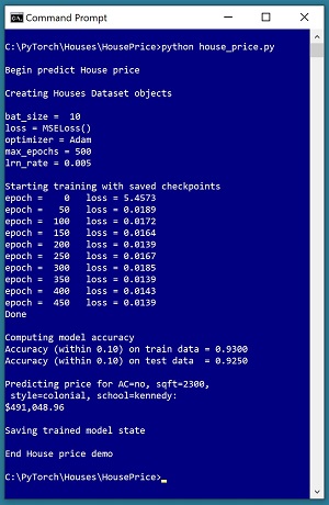
A good way to see where this series of articles is headed is to take a look at the screenshot of the demo program in Figure 1. The demo begins by creating Dataset and DataLoader objects which have been designed to work with the house data. Next, the demo creates an 8-(10-10)-1 deep neural network. The demo prepares training by setting up a loss function (mean squared error), a training optimizer function (Adam) and parameters for training (learning rate and max epochs).
 [Click on image for larger view.] Figure 1: Neural Regression in Action
The demo trains the neural network for 500 epochs in batches of 10 items. An epoch is one complete pass through the training data. The training data has 200 items, therefore, one training epoch consists of processing 20 batches of 10 training items.
During training, the demo computes and displays a measure of the current error (also called loss) every 50 epochs. Because error slowly decreases, it appears that training is succeeding. Behind the scenes, the demo program saves checkpoint information after every 50 epochs so that if the training machine crashes, training can be resumed without having to start from the beginning.
After training the network, the demo program computes the prediction accuracy of the model based on whether or not the predicted house price is within 10 percent of the true house price. The accuracy on the training data is 93.00 percent (186 out of 200 correct), and the accuracy on the test data is 92.50 percent (37 out of 40 correct). Because the two accuracy values are similar, it is likely that model overfitting has not occurred.
Next, the demo uses the trained model to make a prediction on a new, previously unseen house. The raw input is (air conditioning = "no", square feet area = 2300, style = "colonial", school = "kennedy"). The raw input is normalized and encoded as (air conditioning = -1, area = 0.2300, style = 0,0,1, school = 0,1,0). The computed output price is 0.49104896 which is equivalent to $491,048.96 because the raw house prices were all normalized by dividing by 1,000,000.
The demo program concludes by saving the trained model using the state dictionary approach. This is the most common of three standard techniques.
This article assumes you have an intermediate or better familiarity with a C-family programming language, preferably Python, but doesn't assume you know very much about PyTorch. The complete source code for the demo program, and the two data files used, are available in the download that accompanies this article. All normal error checking code has been omitted to keep the main ideas as clear as possible.
To run the demo program, you must have Python and PyTorch installed on your machine. The demo programs were developed on Windows 10 using the Anaconda 2020.02 64-bit distribution (which contains Python 3.7.6) and PyTorch version 1.7.0 for CPU installed via pip. You can find detailed step-by-step installation instructions for this configuration in my blog post.
The House Data
The raw House data is synthetic and was generated programmatically. Although the data is synthetic, it is inspired by the well-known Boston Area Housing Dataset where the goal is to predict the average price of a house in one of 506 towns near Boston, based on 13 predictor variables such as average house age, percentage of minority residents, tax rate and so on. The demo data has a total of 240 items, divided into a 200-item training dataset and a 40-item test dataset. The raw data looks like:
no    1275   bungalow   $318,000.00   lincoln
yes   1100   art_deco   $335,000.00   johnson
no    1375   colonial   $286,000.00   kennedy
yes   1975   bungalow   $512,000.00   lincoln
. . .
no    2725   art_deco   $626,000.00   kennedy
Each line of tab-delimited data represents one house. The value to predict, house price, is in 0-based column [3]. The predictors variables in columns [0], [1], [2] and [4] are air conditioning, area in square feet, style and local school. For simplicity, there are just three house styles and three schools.
House area values were normalized by dividing by 10,000 and house prices were normalized by dividing by 1,000,000. Air conditioning was binary encoded as no = -1, yes = +1. Style was one-hot encoded as "art_deco" = (1,0,0), "bungalow" = (0,1,0), "colonial" = (0,0,1). School was one-hot encoded as "johnson" = (1,0,0), "kennedy" = (0,1,0), "lincoln" = (0,0,1). The resulting normalized and encoded data looks like:
-1   0.1275   0 1 0   0.3180   0 0 1
 1   0.1100   1 0 0   0.3350   1 0 0
-1   0.1375   0 0 1   0.2860   0 1 0
 1   0.1975   0 1 0   0.5120   0 0 1
. . .
-1   0.2725   1 0 0   0.6260   0 1 0
Because the synthetic House data is mixed numeric and categorical and has multiple dimensions, it's not possible to easily display the data in a graph. But you can get an idea of what the data is like by examining the graph in Figure 2. It shows the 200-item training data with the house price as a function of just the house area. Notice the data is quite linear so basic linear regression is a candidate technique. As it turns out, a simple linear regression model on the House data, using just area in square feet, gives 70.00 percent prediction accuracy. This value can be used as a baseline for comparison when evaluating the neural regression prediction accuracy.
 [Click on image for larger view.] Figure 2: Partial House Data
In a non-demo scenario, data preparation can be very time-consuming. It's not uncommon for data preparation to take 80 percent or even more of the total time and effort required to create a prediction model. The demo system presented in this article performs all data preparation as a preprocessing step. An alternative approach is to programmatically perform data normalization and encoding on the fly.
The Overall Program Structure
The overall structure of the demo PyTorch neural regression program, with a few minor edits to save space, is shown in Listing 1. I like to indent my Python programs using two spaces rather than the more common four spaces.
Listing 1: The Structure of the Demo Program
# house_price.py
# PyTorch 1.7.0-CPU Anaconda3-2020.02
# Python 3.7.6 Windows 10

import numpy as np
import time
import torch as T
device = T.device("cpu")

class HouseDataset(T.utils.data.Dataset):
  # AC  sq ft   style  price   school
  # -1  0.2500  0 1 0  0.5650  0 1 0
  #  1  0.1275  1 0 0  0.3710  0 0 1
  # air condition: -1 = no, +1 = yes
  # style: art_deco, bungalow, colonial
  # school: johnson, kennedy, lincoln

  def __init__(self, src_file, m_rows=None): . . .
  def __len__(self): . . .
  def __getitem__(self, idx): . . .

# ----------------------------------------------------

def accuracy(model, ds): . . .

# ----------------------------------------------------

class Net(T.nn.Module):
  def __init__(self): . . .
  def forward(self, x): . . .

# ----------------------------------------------------

def main():
  # 0. get started
  print("Begin predict House price ")
  T.manual_seed(4)
  np.random.seed(4)

  # 1. create Dataset and DataLoader objects
  # 2. create neural network
  # 3. train network
  # 4. evaluate model
  # 5. make a prediction
  # 6. save model
  print("End House price demo ")

if __name__== "__main__":
  main()
It's important to document the versions of Python and PyTorch being used because both systems are under continuous development. Dealing with versioning incompatibilities is a significant headache when working with PyTorch and is something you should not underestimate. The demo program imports the Python time module to timestamp saved checkpoints.
I prefer to use "T" as the top-level alias for the torch package. Most of my colleagues don't use a top-level alias and spell out "torch" many times per program. Also, I use the full form of sub-modules rather than supplying aliases such as "import torch.nn.functional as functional." In my opinion, using the full form is easier to understand and less error-prone than using many aliases.
The demo program defines a program-scope CPU device object. I usually develop my PyTorch programs on a desktop CPU machine. After I get that version working, converting to a CUDA GPU system only requires changing the global device object to T.device("cuda") plus a minor amount of debugging.
The demo program sets the NumPy and PyTorch random number generator seed values so that program runs will be reproducible. The seed value of 4 was used only because it gives representative results.
The demo program defines just one helper method, accuracy(). All of the rest of the program control logic is contained in a main() function. It is possible to define other helper functions such as train_net(), evaluate_model() and save_model(), but in my opinion this modularization approach makes the program more difficult to understand rather than easier to understand.
Defining a House Dataset Class
Serving up batches of data for training a network and evaluating the accuracy of a trained model is a bit trickier than you might expect if you're new to PyTorch. In the early days of PyTorch, the most common approach was to write completely custom code. You can still write one-off code for loading data, but now the most common approach is to implement Dataset and DataLoader objects. Briefly, a Dataset object loads all training or test data into memory, and a DataLoader object serves up the data in batches.
You can think of a PyTorch Dataset as an interface that must be implemented. At a minimum, you must define an __init__() method which reads data from file into memory, a __len__() method which returns the total number of items in the source data, and a __getitem__() method which returns a single data item. There are many design alternatives and no two Dataset class definitions will be the same.
A DataLoader object is instantiated by passing in a Dataset object. The DataLoader object can be iterated, serving up one batch of data at a time. Unlike the Dataset which must be implemented, a DataLoader is ready to use as-is.
The definition of class HouseDataset is shown in Listing 2. In most cases, the structures of the training and test data files are the same and you can use a single Dataset definition for both files. If the structures of your files are different, then you'd have to define two different Dataset classes, or parameterize the Dataset definition.
Listing 2: Class HouseDataset Definition
class HouseDataset(T.utils.data.Dataset):
  # AC  sq ft   style  price   school
  # -1  0.2500  0 1 0  0.5650  0 1 0
  #  1  0.1275  1 0 0  0.3710  0 0 1
  # air condition: -1 = no, +1 = yes
  # style: art_deco, bungalow, colonial
  # school: johnson, kennedy, lincoln

  def __init__(self, src_file, m_rows=None):
    all_xy = np.loadtxt(src_file, max_rows=m_rows,
      usecols=[0,1,2,3,4,5,6,7,8], delimiter="\t",
      comments="#", skiprows=0, dtype=np.float32)

    tmp_x = all_xy[:,[0,1,2,3,4,6,7,8]]
    tmp_y = all_xy[:,5].reshape(-1,1)

    self.x_data = T.tensor(tmp_x, \
      dtype=T.float32).to(device)
    self.y_data = T.tensor(tmp_y, \
      dtype=T.float32).to(device)

  def __len__(self):
    return len(self.x_data)

  def __getitem__(self, idx):
    preds = self.x_data[idx,:]  # or just [idx]
    price = self.y_data[idx,:]
    return (preds, price)       # tuple of matrices
The __init__() method begins by reading all data from file into memory as a matrix using the NumPy loadtxt() function:
  all_xy = np.loadtxt(src_file, max_rows=m_rows,
    usecols=[0,1,2,3,4,5,6,7,8], delimiter="\t",
    comments="#", skiprows=0, dtype=np.float32)
The synthetic House data contains both predictor values and price-to-predict values in the same file, so both can be read at the same time. A slightly less efficient alternative is to read the predictor values with one call to loadtxt() and then read the values-to-predict with a second call.
Python has dozens of ways to read a text file into memory, but using loadtxt() is the technique I usually prefer. Some of my colleagues favor using the NumPy genfromtxt() or fromfile() functions, or the Pandas read_csv() function. The data is read into a NumPy matrix as float32 values which is the default floating point numeric type for PyTorch.
After all the data has been read into memory as a NumPy matrix, the predictor rows and the price-to-predict rows are extracted into separate matrices and then converted to PyTorch tensors:
  tmp_x = all_xy[:,[0,1,2,3,4,6,7,8]]
  tmp_y = all_xy[:,5].reshape(-1,1)

  self.x_data = T.tensor(tmp_x, \
    dtype=T.float32).to(device)
  self.y_data = T.tensor(tmp_y, \
    dtype=T.float32).to(device)
The "[:,[0,1,2,3,4,6,7,8]]" syntax means "a matrix from all rows, all columns except column 5." The "[:,5]" syntax means "a vector from all rows, just column 5." The reshape(-1,1) function converts the vector into a matrix with one column. For regression problems, PyTorch requires a two-dimensional matrix of target values rather than a one-dimensional vector. The strange -1 argument in reshape() is a PyTorch idiom that means "PyTorch interpreter, you figure out the correct value for the number of rows."
Many of the examples I've seen on the internet convert the input data to PyTorch tensors in the __getitem__() method rather than in the __init__() method. Because conversion to tensors is a relatively expensive operation, it's usually better to convert the data once in __init__() rather than repeatedly in the __getitem__() method.
At this point in the program execution, self.x_data is a two-dimensional tensor matrix with eight columns. In practice, you usually need to experiment a bit and examine objects with code like:
print("x_data is ")
print(self.x_data)
print(self.x_data.shape)
input()  # pause execution
Alternatively, if you're using a powerful IDE such as Visual Studio to write your code, you can set an execution breakpoint and examine variables.
The implementation of the Dataset __len__() method is simple:
  def __len__(self):
    return len(self.x_data)
The Dataset object needs to be able to return the number of items it has so that the DataLoader object that uses the Dataset can determine when all data items have been processed once, and then start a new epoch. The Dataset m_rows parameter is passed to the loadtxt() max_rows parameter. If max_rows has value None, then loadtxt() will load all lines of the source data file. So, if you omit the m_rows parameter when instantiating a Dataset object, the default parameter value of None will be used, which will be passed to loadtxt() and all lines of data will be read into memory. Therefore, the __len__() method needs to return len(self.x_data), the actual number of lines of data read, rather than m_rows, which could be None. The moral of this story is that even simple-looking PyTorch statements must be thought through very carefully.
The Dataset __getitem__() method is defined as:
  def __getitem__(self, idx):
    preds = self.x_data[idx,:]  # or just [idx]
    price = self.y_data[idx,:]
    return (preds, price)       # tuple
The method returns one data item as a tuple where the first element is a matrix of predictor values and the second element is a matrix of target values. A common alternative is to return the two matrices as a Dictionary object, for example:
sample = {
  'predictors' : preds,
  'prices' : price
}
return sample
To extract values from a Dataset, you normally don't call the __getitem__() method directly. If you access a Dataset object using indexing, or using the built-in Python enumerate() function, the __getitem__method() is automatically called.
Testing the Dataset
It's good practice to test a Dataset and DataLoader before trying to use them to train a neural network. The short program in Listing 3 shows an example. The test program sets up a Dataset with just the first five items from the 200 normalized and encoded House training data. Then the tester iterates twice through the five items, in batches of size two items. Therefore, each epoch serves up batches of size 2, 2 and 1 items. See the screenshot in Figure 3.
Listing 3: Testing the Dataset using a DataLoader
# test_dataset.py
# PyTorch 1.7.0 CPU
# Python 3.7.6

import numpy as np
import torch as T
device = T.device("cpu")

class HouseDataset(T.utils.data.Dataset):
  # see Listing 2

T.manual_seed(0)

src = ".\\Data\\houses_train.txt"
train_ds = HouseDataset(src, m_rows=5)
train_ldr = T.utils.data.DataLoader(train_ds,
  batch_size=2, shuffle=True)
for epoch in range(2):
  print("\n\n Epoch = " + str(epoch))
  for (bat_idx, batch) in enumerate(train_ldr):
    print("------------------------------")
    X = batch[0]  # batch is tuple of two matrices
    Y = batch[1]
    print("bat_idx = " + str(bat_idx))
    print(X)
    print(Y)

print("\nEnd test ")
The test program assumes the data files are in a subdirectory named Data. The PyTorch DataLoader class is defined in the torch.utils.data module. A DataLoader has 10 optional parameters but in most situations you pass only a (required) Dataset object, a batch size (the default is 1) and a shuffle (True or False, default is False) value. The shuffle parameter controls whether the data items should be served up in random order, typically during training, or in sequential order, typically during model evaluation.
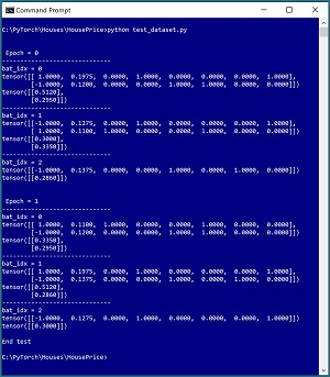 [Click on image for larger view.] Figure 3: Testing the Dataset and DataLoader
The core statement that uses the Dataset and DataLoader is:
for (bat_idx, batch) in enumerate(train_ldr):
  . . .
The enumerate() function is a built-in Python mechanism to walk through objects that are iterable, which includes DataLoader objects. The return value is a tuple where the first value, "bat_idx," is the 0-based batch index and the second value, "batch," is a tuple where the first element is a matrix of predictor values and the second element is a matrix of target house prices. The short test program is just a beginning and you should test any Dataset object you define by iterating through all data items, with both the training and test data, and with the shuffle parameter set to both True and False.
Wrapping Up
Neural regression is more complicated than classical statistics regression techniques, but neural regression is more powerful in the sense that it can deal with complex, non-linear data. The two major disadvantages of neural regression are:
- The technique requires lots of training data
- Resulting prediction models are susceptible to overfitting
In some problem scenarios, using an ensemble technique that combines a classical statistics regression model with a neural regression model can be an effective strategy.
The example code presented in this article can be used as a template for most neural regression problems. One exception is a scenario where your training data is too large to fit entirely into memory. Fortunately, these situations are relatively rare. For huge data files, the most usual approach is to define a Dataset object where the __init__() method reads part of the huge file into a buffer, and then when all of the buffer data has been processed by calls to the __getitem__() method, a program-defined reload() method refills the buffer with the next block of data.